Chapter 2. Integrating inclusiveness in the Going for Growth framework1
This chapter discusses how the Going for Growth framework is extended to fully take into consideration inclusiveness as a policy objective, alongside employment and productivity growth. It first provides a broad picture of inclusiveness trends across OECD and selected non-OECD countries, focusing on income distribution and inequality outcomes. The chapter then offers a comprehensive assessment of policy challenges related to inclusiveness and potential remedies reflected in the formulation of Going for Growth reform priorities.
Main findings
-
A new extended Going for Growth framework is used to identify country-specific reform priorities based on their ability to boost growth and make it more inclusive. The framework for selecting policy priorities now considers inclusiveness as a prime objective, alongside productivity and employment.
-
Such priorities are derived from a combined quantitative assessment based on cross-country comparisons in growth and inclusiveness outcomes and policy settings, along with a qualitative assessment based on country expertise.
-
Metrics of inclusiveness are based on a dashboard of indicators encompassing a number of income and non-income dimensions such as inequality and poverty, job quantity and job quality, along with labour market inclusion of vulnerable groups, gender gaps and equity in education, as well as health outcomes.
-
There is significant scope for selecting priorities that can exploit synergies between the pursuit of growth and inclusiveness:
-
Almost half of the 2017 Going for Growth priorities identified under the extended framework would make growth more inclusive in the sense that the corresponding reforms would boost growth and reduce income inequalities.
-
Considering that in a number of areas pro-growth policies may potentially conflict with the inclusiveness objective, the integration of the latter in the selection of policy priorities further raises the importance of considering reform packages to achieve strong and inclusive growth.
-
-
In seeking to make growth more inclusive, governments should focus on the following policy areas:
-
Ensuring broad access to quality education and upskilling. Education shapes each individual’s life chances and is closely related to skills and training, which in turn increasingly determines people’s ability to earn a decent living. Policy reforms need to address the needs of young people from pre-school to university, so that they get the best start in life and the support they need throughout their education. The focus is on enhancing equality of opportunities and securing adaptability of the workforce to changing demand for skills.
-
Lifting the quantity and the quality of jobs and addressing labour market insecurity and segmentation. Policy reforms are identified with a view to creating quality jobs while integrating specific socio-demographic groups that are underrepresented in the workforce, most notably young people and women. At the current juncture, governments must minimise the risk of vulnerable youth – such as early school leavers who are neither employed nor in education or training (NEETs) – permanently facing a difficult access to the labour market. Creating more and better jobs also requires tackling labour market duality and segmentation, including informality in the case of emerging economies.
-
Enhancing the effectiveness of tax and transfer systems in reducing income inequality and poverty, taking into account equity and efficiency objectives. Many countries have room for making their tax and transfer systems more efficient with no adverse distributional implications. This includes designing social transfers with a view to protecting individuals and families who need it most while ensuring that work pays for those at the low-end of the income distribution and for women, as well to limiting tax breaks and allowances that disproportionately benefit high-income households.
-
Introduction
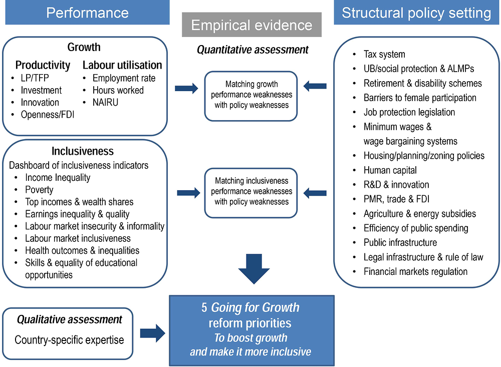
1. This chapter presents and discusses an extended framework integrating inclusiveness in Going for Growth.2 It is applied for the first time to identify the 2017 country-specific reform priorities formulated in Chapter 3. The extended framework incorporates priorities against performance metrics of productivity, employment and inclusiveness. Adapting the priority selection process along these lines reflects the empirical evidence clearly signalling that higher growth is not systematically associated with rising living standards for the vast majority of citizens. In particular, the dispersion of disposable incomes (i.e. after taxes and social transfers) has been on the rise during the past 30 years (Atkinson, 2015; OECD, 2008; 2011a; 2015b).3 Rising income inequality is not only the reflection of rising top incomes, but also that of falling or stagnating bottom incomes, potentially dampening educational opportunities and social mobility. Moreover, rising inequality has played out against a global slowdown in productivity growth which, at least in many advanced economies, predates the crisis (OECD, 2016a; 2016b). Policy makers thus need to address the twin challenge of slowing productivity and rising inequality.
2. The revised Going for Growth priority-setting framework continues to build on matching relative weaknesses in performance with relative weaknesses in policy settings, covering now inclusiveness alongside productivity and employment growth. The integration of inclusiveness is based on a dashboard of indicators encompassing a number of income and non-income dimensions such as inequality and poverty, job quantity and job quality along with labour market inclusion of vulnerable groups, gender gaps and equity in education. The quantitative assessment delivered by the matching exercise is complemented with a qualitative assessment based on country expertise, with a view to capturing potential policy imperatives in fields not covered by the indicators as well as to tailoring country-specific reform strategies to country-specific context and circumstances.
A flexible framework for integrating inclusiveness in the identification of Going for Growth priorities
A dashboard of inclusiveness indicators
3. The integration of inclusiveness in the identification of country-specific reform policy priorities builds on a dashboard of indicators encompassing various income and non-income dimensions of inequality and, more broadly, inclusiveness. These indicators are used to assess countries’ relative outcomes in associated areas, considering levels and changes over time. Figure 2.1 presents the dashboard and associated indicators while the Annex provides the data on a country-by-country basis. Since the various dimensions of inclusiveness cannot adequately be captured by a single measure that can then be broken into sub-components, there is no clear analytical framework for linking together the various indicators, as can be done for GDP per capita, productivity and employment.
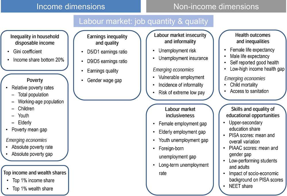
4. The dashboard covers standard measures of household disposable income inequality along with some of its components (e.g. disposable income inequality at different points of the distribution, wage inequality among workers); as well as poverty measures (e.g. relative poverty for total population and for different demographic groups, absolute poverty being used for emerging economies). Labour market indicators feature prominently in the dashboard, reflecting the importance of labour market status and labour income as a major driver of inequality and inclusion in society, in addition to being a driver of growth. This also reflects that evidence on the link between policies and outcomes is relatively more abundant in this area. Overall, labour market indicators cover job quantity and job quality. Job quality draws on the OECD Job Quality framework, encompassing earnings quality and labour market insecurity, with a complementary focus on informality and risk of extreme low pay in emerging economies.4
5. The dashboard also emphasises labour market inclusiveness, i.e. the integration of women (and, more broadly, the gender divide), youth, elderly and migrants in the labour market. It includes selected non-income dimensions, first and foremost in the area of skills and equity in education, as this in turn increasingly determines peoples’ ability to earn a decent living and participate in society, on top of being a major driver of productivity growth (OECD, 2016a). Associated outcomes are measured on the basis of PISA and PIAAC data, hence covering both youth and adults; finally, the dashboard covers available measures of health outcomes and health inequalities.5 The specific indicators have been chosen to cover both the overall degree of inequality in each income and non-income dimension, as well as the degree of horizontal inequalities; that is, within each of those dimensions, inequalities across socio-demographic groups based on gender, age, migration status and education.
6. Inequality is mainly assessed from a static perspective rather than from a dynamic perspective, which would imply covering inequality throughout the lifecycle and across generations. It is also mainly assessed in terms of outcomes rather than opportunities. This essentially reflects the lack of data on a cross-country comparable basis as well as the limited available evidence between outcomes and policies in this area. As an attempt to partly overcome associated limitations, the dashboard includes an assessment of inequality of educational opportunities with a view to coming closer to issues of intergenerational social mobility. This is measured by the estimated impact of students’ socio-economic background on PISA scores. Overcoming data constraints is key to identifying robust empirical relationships between the various income and non-income dimensions of well-being and policies, as well as to ensure their responsiveness to policy intervention. This is work in progress at the OECD and will gradually be integrated in Going for Growth.6
Matching performance weaknesses with policy weaknesses in the inclusiveness dimension
7. The Going for Growth priority-setting process is based on matching performance weaknesses and policy weaknesses, taking the OECD average outcome as a benchmark. In this regard, the priority-setting extended to the inclusiveness dimension follows the same logic of the priority-setting implemented so far, focused on the growth dimension only (see Chapter 1 and past issues of Going for Growth). The identification of reform priorities and the formulation of underlying recommendations build on a “mixed” approach under which the quantitative assessment delivered by the matching between outcome indicators and policy indicators is complemented by a qualitative assessment so as to tailor reform strategies to country-specific context and circumstances (Figure 2.2). Such a qualitative assessment is based on local expertise, that is, in consultation with OECD country specialists. This allows also for capturing reform imperatives in policy areas which cannot be easily quantified and therefore which are not covered by the quantitative matching.
8. Inclusiveness indicators included in the dashboard are matched with corresponding policy indicators, where empirical research has shown a robust link, to determine where performance weaknesses are a potential reflection of policy weaknesses.7 For this exercise, the matching focuses mainly on the inclusiveness impact of growth-friendly policies, implying that it leaves out inequality-reducing tax and transfer reforms.8 This is because the empirical evidence on the growth impact of such reforms is still limited.
9. Thus, at this stage the framework builds on the extensive empirical research on the effects of pro-growth structural policies on income inequality and, more broadly, inclusiveness outcomes (see Chapter 2 in OECD, 2015a, for a summary of the literature). In particular:
-
Empirical evidence on the impact of structural reforms on household disposable incomes across the distribution, hence on income inequality (OECD, 2011a; Causa et al. 2015; 2016) and on wage dispersion among employees (OECD, 2011a; Braconier and Ruiz-Valenzuela, 2014). For example, the level of long-term unemployment benefits and public spending on in-kind family benefits (policy indicators) are matched with disposable income inequality when inequality is assessed through measures that emphasise the bottom of the distribution (outcome indicator). The share of population with tertiary education (policy indicator) is matched with a measure of wage inequality based on the ratio of the ninth decile (highest wages) over the fifth decile or median wages (outcome indicator).
-
Empirical evidence on the impact of pro-growth reforms on labour market insecurity, informality and labour market inclusion of specific population groups (Gal and Theising, 2015; De Serres and Murtin, 2014). For example, the employment rate of women (performance) is matched with public spending on in-kind family benefits (related policy). Youth employment (performance) is matched with public spending on active labour market policies (ALMPs; related policy). Long-term unemployment and incidence of informality (performance) are matched with employment protection legislation (EPL) for regular contracts (related policy). Labour market insecurity (performance) is matched with coverage of unemployment benefits and social assistance (related policy).
-
Empirical evidence on the impact of pro-growth reforms on intergenerational social mobility (Causa and Johansson, 2009). For example, the impact of socio-economic background on PISA performance (performance) is matched with spending on childcare and pre-school (related policy).
-
Empirical evidence on the impact of pro-growth reforms on poverty (Marx et al., 2015; World Bank, 2015).9 For example, relative poverty (performance) is matched with income levels for families relying on minimum-income, safety-net benefits or with full-time minimum wage employment (related policy).
10. Figure 2.3 gives an example of the matching between household disposable income inequality and public spending on services and in-kind family benefits (which covers for instance direct financing of providers of childcare and early education facilities). Countries are benchmarked against the OECD average by standardising both performance and outcome indicators to have cross-country mean zero and standard deviation of one, with positive values representing more inclusiveness-friendly positions. Accordingly, reforming in-kind family benefits is a candidate priority for those countries falling into the lower-left quadrant of the figure, i.e. those that exhibit higher than OECD average disposable income inequality and lower than OECD average public spending on in-kind family benefits. Not all candidate priorities ultimately correspond to actual priorities, which is why for example some countries do not feature a priority in the area of in-kind family benefits even though they fall into the lower-left quadrant of Figure 2.3. Country-specific expertise is used to determine whether a candidate reform priority is indeed a pressing challenge in the given country context; and, if yes, for tailoring the specific recommendation to the specific nature of the challenge at stake.
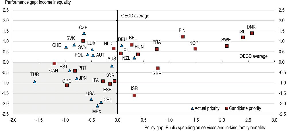
How to read this figure: The vertical axis displays cross-country performance in terms of income inequality (measured by a bottom-sensitive Atkinson inequality index with parameter -4, see Causa et al., 2016). The horizontal axis displays cross-country policy-setting in terms of public spending on services and in-kind family benefits in per cent of GDP (among other a measure of access to childcare and early childhood education). Both indicators have been standardised by re-scaling them so that each has a cross-country mean of zero and a standard deviation of one, with positive numbers representing positions more inclusiveness-friendly than the OECD average. The scatter plot is thus divided into four quadrants, depending on whether a country’s policy-performance pairing is below or above the average policy or performance score. Hence, reforming in-kind family benefits is a candidate priority for countries falling into the lower-left quadrant (e.g. Turkey), where the policy and corresponding performance indicator are both below the OECD average. Countries marked by a triangle have expanding access to childcare and early childhood education among their Going for Growth priorities (see Chapter 3).
11. The matching between performance and policies is less comprehensive in the case of inclusiveness outcomes compared to the well-established case of productivity and employment. As a result, not all indicators included in the dashboard can be matched with policies. Such is the case of various dimensions of risk of social exclusion for specific demographic groups, for instance the share of youth that are NEET, as well as inequality in health.
12. However, even in the absence of a matching between outcome and policies, dashboard indicators remain useful and are used in the priority selection process. Relatively high levels or increases in such indicators can signal that countries may face a potential weakness in associated areas. When this is the case, country experts can judge the extent to which this can be traced to country-specific policy weaknesses and hence to policy levers.
Principles of the priority-setting process
13. The priority-setting process can then be summarised as follows:
-
Five policy priorities are identified from the combined quantitative matching of performance and policy weaknesses in the growth and equity dimensions with the qualitative assessment by country experts. The relative emphasis put on labour productivity, labour utilisation and inclusiveness in the selection of the five priorities varies across countries and is established with country experts. In doing so, it takes into consideration how distant from good practice a country is in the respective performance and related policy areas as well as country-specific circumstances and expert judgment (see also Box 1.2 in Chapter 1).
-
Policy reform complementarities between equity and growth objectives arising from the matching between performance and policy weaknesses are given priority when evidence suggests that such reforms may help address inclusiveness concerns:
-
That is overwhelmingly the case for education reforms aimed at increasing equality of opportunity, especially when the focus is on early childhood. Such reforms are fundamental from an inclusiveness perspective, even though their benefits are likely to materialise over the medium-term and inter-generationally. An example for a country that suffers from low equity in education and/or weak labour market inclusion of women would be to enhance access to quality childcare for children from disadvantaged backgrounds, if childcare facilities are relatively scarce or unaffordable.
-
That is also the case for reforms aimed at reducing the level and duration of unemployment and at enhancing the labour market integration of vulnerable groups. The benefits from these reforms may materialise over a shorter horizon compared to education reforms.10 An example for a country that suffers from severe youth unemployment would be to improve co-ordination between education and ALMPs and to strengthen apprenticeships and vocational education and training (VET) if spending on such areas is insufficient or inefficient.
-
-
Policy reform packages are designed to mitigate adverse effects arising from potential trade-offs between growth and inclusiveness when evidence suggests that a given pro‐growth reform may increase inequality in a country that is already facing challenges in this area:11
-
That may for instance occur in the case of tax and transfer reforms, as there may be tensions between raising economic incentives and redistributing income. Examples include pro-growth tax reforms shifting the tax burden from income to consumption, as this may raise inequality in the short run.12 In this instance, reform packages can be designed to be consistent with equity goals by expanding or introducing well-targeted cash transfers – taking into account growth and redistribution objectives – or by reducing tax breaks that disproportionately benefit the rich, such as for owner-occupied housing or retirement savings.
-
-
The priority-setting process does not aim at systematically avoiding trade-offs between growth and equity objectives; some trade-offs may remain when, in the judgement of the country experts, the outcome of growth-oriented reforms is deemed to prevail over the outcome of equity-oriented reforms because of country-specific context, including social preferences. In practice, few such trade-offs arise, as discussed below (see also Chapter 1 and Chapter 3). Countries exhibit large room for improving their pro-growth policy stance in an equity-friendly way and concerns about reform-driven inequality increases cannot be used as arguments to hold back on reforms.
14. The overall distributional effects of some pro-growth reform priorities are sometimes ambiguous and potentially negligible, as their impact may operate through different offsetting channels. As a result, a number of Going for Growth priorities cannot be unambiguously classified as inclusive or not. Such is the case of reforms aimed at stimulating innovation and technological progress, including measures to reduce barriers to competition, firm entry and entrepreneurship. Progress along these lines is fundamental to spur productivity growth but may put further pressure on the relative demand for skilled workers through skill-biased technical change, and hence contribute to rising wage inequality among workers. At the same time, insofar as such reforms also contribute to job creation, they are likely to counteract reform-driven increases in wage dispersion, with an overall ambiguous effect on disposable income inequality.13, 14 Furthermore, and in a longer-term perspective, competition and innovation policies may also contribute to enhance equity, for instance if they lead to a reduction in firms’ rents and undermine the market dominance of incumbents, while promoting social mobility (OECD, 2016a). Indeed, recent evidence suggests that intergenerational income mobility increases with the degree of entrepreneurship and innovativeness in the economy (Aghion et al., 2015; 2016).
159. The approach spelled-out in this section is implemented in the selection of the 2017 Going for Growth priorities which are presented in the Country Notes (Chapter 3). This approach will progressively evolve as progress is being achieved in terms of understanding the effects of policy reforms on growth and inclusiveness, and, going further, additional policy objectives such as environmental sustainability will be included.
A first look at inclusiveness: cross-country patterns in income distribution
The big picture: income inequality across countries and over time
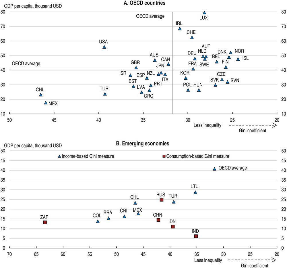
16. The integration of inclusiveness in the identification of Going for Growth priorities starts with an overview of countries’ relative positions in the area of income inequality. This is the fundamental building block of the framework and a key concern among policy makers. The income concept used for this purpose is that of household disposable income for the total population, considered as the best proxy of households’ economic resources defined by internationally agreed standards and computable across the income distribution.15 One widely-used measure of income inequality is the Gini coefficient, owing to its broad availability on a consistent basis across countries.16 The simultaneous assessment of cross-country differences in income inequality and GDP per capita delivers the following main insights (Figure 2.4):
← 1. The Gini index measures the extent to which the distribution of disposable income among households deviates from perfect equal distribution. A value of zero represents perfect equality and a value of 100 extreme inequality. GDP per capita is measured in 2015 purchasing power parities (PPP). Data for Gini coefficients refer to 2011 for India and South Africa; 2012 for China, Japan, New Zealand, and the Russian Federation; 2014 for Australia, Brazil, Colombia, Costa Rica, Finland, Hungary, Israel, Korea, Mexico, the Netherlands, and the United States; and 2013 for the rest. Data for GDP per capita refer to 2015.
Source: OECD, Income Distribution and National Accounts Databases; World Bank, World Development Indicators Database.
-
While there is no strong link between GDP per capita and income inequality, cross-country patterns related to different social welfare models and development stages prevail.17 In particular, emerging economies all display high inequality in conjunction with low GDP per capita.18
-
English-speaking countries, in particular the United States and, to a lesser extent, the United Kingdom and Australia, are among the countries with the highest GDP per capita, but at the same time with the highest inequality. By contrast, Central and Eastern European countries, such as Poland, Slovenia and the Slovak Republic, are characterised by relatively low income inequality and relatively low GDP per capita, reflecting a post-communist transition process.
-
Relatively high GDP per capita are accompanied by low income inequality among highly egalitarian Nordic European countries such as Denmark and Norway, but also, to a lesser extent, of some Continental European countries, e.g. Austria and the Netherlands.
17. Cross-country patterns in income inequality depend on how inequality is measured and in particular on whether the emphasis is on incomes in the middle of the distribution or on incomes in the bottom of the distribution (Figure 2.5):
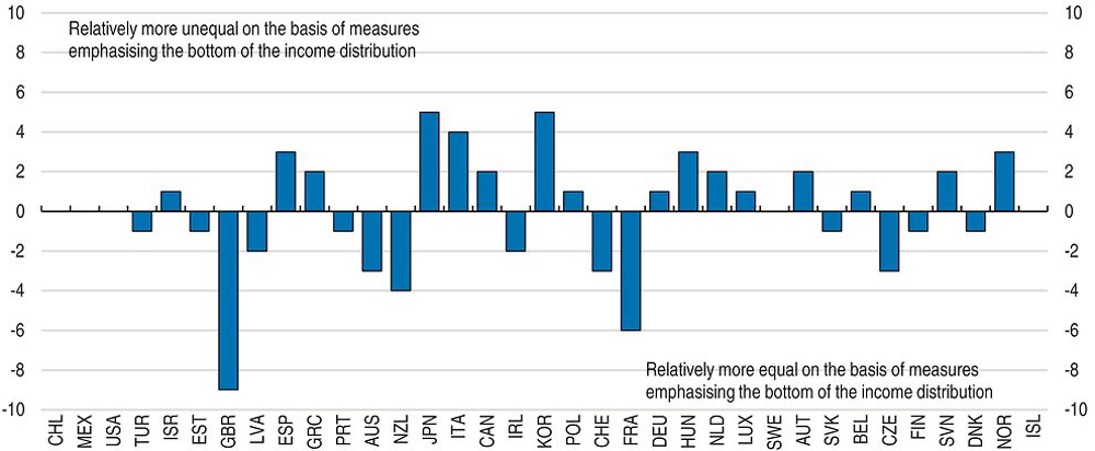
← 1. See note to Figure 2.4 for country and year coverage.
← 2. Measured by the share of total household disposable income accruing to the bottom 20%. Overall inequality is measured by the Gini coefficient.
Source: OECD, Income Distribution Database.
-
Korea and Japan are ranked respectively as the 18th and 14th most unequal OECD countries according to the Gini coefficient, but as the 13th and 9th most unequal countries according to the income share accruing to the bottom 20%. This reflects widespread income dispersion at the low end of the distribution and high poverty.19
-
In the direction of less inequality, the United Kingdom moves 9 places and France moves 6 places in the ranking by emphasising relatively more the bottom of the income distribution, a likely reflection of the emphasis of income redistribution to the low-end of the distribution.
-
For most emerging economies, the two measures result in fairly similar rankings.20 Inequalities in emerging economies are most often driven by regional divides, in particular between rural and urban areas.
18. Since the mid-2000s, overall income inequality, as measured by the Gini coefficient after taxes and transfers, has been stable on average across the OECD and has decreased in around half of the emerging economies covered in this paper (Figure 2.6).21 Countries have experienced different distributional developments, in part reflecting differences in the depth of the crisis, as well as differences in the sources of changing income inequality:
← 1. For Panel A and B data refer to 2003-12 for Japan and New Zealand; 2004-14 for Australia, Finland, Mexico, and the United States; 2005-13 for Denmark and Poland; 2005-14 for Hungary, Israel, and the Netherlands; 2006-13 for Chile; 2006-14 for Korea; 2009-12 for Switzerland; and 2004-13 for the rest. A break in the series in 2011-12 for most countries is accounted for by computing the total change as the sum of the change before and after the break, using a year for which the two series overlap. For Panel B household disposable incomes have been deflated by the consumer price index. For Panel C data refer to 2004-11 for India; 2004-12 for the Russian Federation; 2004-13 for Lithuania and Turkey; 2005-13 for China; 2006-11 for South Africa; 2006-13 for Chile; and 2004-14 for the rest. Income inequality measures are based on consumption for some emerging economies, see Figure 2.4, Panel B.
Source: OECD, Income Distribution Database; World Bank, PovcalNet.
-
In 7 OECD countries, the Gini coefficient decreased and in 5 countries it increased by more than 0.2 percentage points per year, while most countries in-between these two groups experienced relatively little change in the Gini coefficient (Figure 2.6, Panel A). Among advanced OECD countries, the most populated ones, in particular the United States, experienced increases in inequality, while mainly the least populated ones experienced decreases, with Portugal and Switzerland exhibiting the largest decline in the Gini coefficient. This may explain the popular perception of a widespread rise in income inequality among advanced countries, insofar as a majority of citizens live in inequality-increasing countries.22
-
In most countries where inequality declined, such as in Turkey and Poland, this reflected real disposable incomes growing across the whole distribution but relatively more among less affluent than more affluent households (Figure 2.6, Panel B). Portugal stands out as having experienced the strongest decline in the Gini coefficient yet this reflected real disposable incomes declining across the entire income distribution but relatively more at its high end.
-
In some countries where inequality increased, such as Slovenia and Spain, this reflected real disposable incomes declining among poor households and rising among middle class and more affluent households; while in the United States it reflected real disposable incomes declining among all income groups except the most affluent households (Figure 2.6, Panel B). Greece stands out as rising inequality reflected real disposable incomes declining across the entire income distribution but relatively more at its low end.
-
Emerging economies experienced heterogeneous distributional developments, both between countries as well as within countries, that is, between rural and urban areas (Figure 2.6, Panel C). Inequality declined by more than 0.5 percentage points per year in Brazil while it increased by more than 0.5 percentage points per year in Indonesia, especially in urban areas. The People’s republic of China, (hereafter ‘China’), also experienced a rise in urban inequality while rural inequality declined.
-
Cross-country patterns indicate some degree of “convergence” in income inequality: inequality tended to decrease (increase) in countries with relatively high (low) initial inequality (Figure 2.6, Panel A and C).23
The profile of income inequality, poverty and its potential impact on the growth process
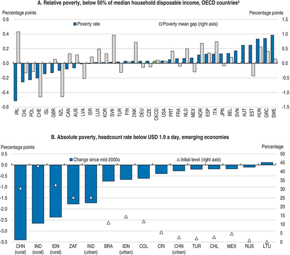
19. A broad overview of poverty developments since the mid-2000s shows that in the majority of advanced countries vulnerable households have experienced increased income hardship. The risk of falling below the relative poverty threshold of 50% of median disposable income has increased in 2 out of 3 OECD countries and in more than half of OECD countries, those that are poor have been falling behind relative to the poverty threshold (Figure 2.7, Panel A),24 which signals rising inequality at the low end of the distribution. To a large extent, this situation reflects crisis-driven falls in market incomes, for instance in those countries having experienced strong rises in unemployment. However, rising poverty rates and gaps also took place in countries that were relatively less hit by the crisis and where employment has been growing for several years now, such as Sweden and Hungary.
20. Increased income hardship among the poor may also signal some weakening of the welfare state, i.e. that public redistribution through taxes and cash transfers did less to counteract the rise in market-driven economic vulnerability. This is likely to reflect the lower effectiveness of tax and transfers in reducing income inequality which has been observed over the second phase of the crisis, as governments introduced fiscal consolidation programmes and phased-out fiscal benefits granted to households over the first phase of the crisis (OECD, 2015b, Chapter 3). The bottom line is that in many advanced countries poorest households have been increasingly falling behind the rest of society, to a large extent reflecting adverse developments in market incomes at the bottom of the distribution, in particular over the crisis period; but also, over the most recent period, a weakening of governments’ income redistribution.
21. Rising inequalities at the bottom of the income distribution is not only a matter of concern from an inclusiveness perspective, but also from a growth perspective. Indeed, theory and empirical evidence suggests that inequality in the bottom of the distribution and poverty have a detrimental impact on economic growth. From a theoretical perspective, under-investment in human capital by the poorest of society in the presence of financial market imperfections results in low intergenerational social mobility due to talent misallocation; hence ultimately lower efficiency and aggregate output.25 From an empirical perspective, evidence shows that the profile of income inequality matters for economic growth. Voitchovsky (2005) finds that while income inequality in the bottom of the distribution harms growth, income inequality in the top of the income distribution has the opposite effect.26
22. Recent work by Aghion et al. (2015) goes further and provides some support to the Schumpeterian view whereby the rise in top income shares is partly related to innovation-led growth, where innovation itself fosters social mobility at the top through creative destruction. This does not imply that the surge in top incomes documented over the last decades (Piketty, 2013; Ruiz and Woloszko, 2015) should not be a case for policy concern. The point is that high inequality in the top of the income distribution may be less of a concern if it is the reflection of social mobility across generations, whereas it should be both an equity and an efficiency concern if it is the reflection of rent-seeking behaviour and cronyism. From a policy perspective, when rents reflect policy distortions that allow high-performing incumbent firms to erect artificial barriers to competition, reforms aimed at reassessing competition at the top of the productivity distribution may be desirable on both growth and equity grounds.
23. The case for focusing policy design and action on enhancing outcomes and opportunities among the poorest households is even stronger for emerging economies because these countries have not yet eradicated absolute poverty. Considerable progress has been achieved in this area, one of the key objectives of the Millennium Development Goals (MDGs), still in some countries absolute poverty remains prevalent, especially in rural areas; for instance around a quarter of Indian rural population lives below the poverty line (Figure 2.7, Panel B). In turn, the detrimental effect of poverty on economic growth and the development process for emerging economies has been widely documented and discussed (e.g. Ravallion, 2012). Underlying mechanisms reflect not only the human capital channel but also other deprivation-related channels such as the detrimental impact of poor nutritional status on productivity. While absolute poverty is being reduced in emerging economies, inequalities are sometimes increasing at the same time or not being reduced at a significant pace (see Figure 2.6 and Table 2.A1.2). Under current relatively weak growth rates compared to previous decades, a more rapid decline in inequality is needed to reach the poverty-reduction goal by 2030 (World Bank, 2016). Achieving shared prosperity is also needed to sustain the ongoing development of a middle class in emerging economies, which is key to foster growth and economic stability.
← 1. Relative poverty is defined as the share of individuals with equivalised disposable income less than 50% of the median for the entire population. The poverty gap is the distance between the poverty threshold and the mean income of the poor, expressed as a percentage of the poverty threshold.
2. For Panel A see note to Figure 2.4 for time coverage. For Panel B data refer to 2003-13 for Chile; 2004-2011 for India; 2004-12 for Lithuania and the Russian Federation; 2004-13 for Turkey; 2005-13 for China; 2006-11 for South Africa; and 2004-14 for the rest.
Source: OECD, Income Distribution Database; World Bank, PovcalNet.
24. The challenge of raising outcomes and opportunities among the most vulnerable households requires differential approaches, first of all between advanced and emerging economies but also depending on country-specific circumstances. For example among advanced countries, both poverty and inequality at the bottom of the income distribution have increased substantially in Sweden, albeit from a relatively low level, while GDP per capita and average household income were growing. Poverty and inequality also rose in Greece, already from a relatively high level, while GDP per capita and average household income have collapsed during the crisis. Therefore, policy reform strategies differ across countries, depending on countries’ starting point and the drivers of distributional changes, but also on social preferences and their evolution over time (for instance adverse distributional changes can reflect policy choices, e.g. countries starting with low inequality may increasingly tolerate rising inequality when the growth objective prevails the equity objective; see next section).
Going beyond income distribution: inclusiveness challenges and potential policy remedies
25. While using measures of income inequality and poverty provides a sense of the magnitude of the inclusiveness challenge in individual countries, the selection of policy priorities is based on an analysis of performance along various dimensions of inclusiveness, going beyond income distribution. The broad outcome of this exercise is outlined in this section. The discussion emphasises the various challenges that countries face in making growth more inclusive. A complete and detailed assessment of the whole set of policy priorities and underlying recommendations for each country is found in Chapter 3.
26. Overall, almost half of Going for Growth priorities are inclusive in the sense that those would reduce income inequality (Figure 2.8, Panel A). That includes foremost human capital priorities (Figure 2.8, Panel B), i.e. policies that improve people’s access to education and training. Associated recommendations are frequent among both advanced and emerging economies. Inclusive priorities in the area of social benefits and ALMPs are also predominant, especially among OECD countries (Figure 2.8, Panel B). Associated reforms would allow for addressing labour market insecurity from unemployment and inadequate social safety nets, especially among vulnerable groups. Likewise, priorities to reform job protection legislation are considered to be inclusive when the objective is to reduce labour market dualism and/or informality.27
27. Making growth more inclusive may in principle involve policy trade-offs, which may not be systematically avoided. In practice, however, across OECD countries less than one tenth of Going for Growth priorities – those identified through the combined quantitative and qualitative (i.e. based on country expertise) assessment – are classified as having clear adverse equity implications because they could increase income inequality (Figure 2.8, Panel A). Trade-offs may arise in the case of some tax and benefit reforms, such as shifting from direct to indirect taxes or reducing marginal income tax rates. The few recommendations in this area are to be found among advanced economies only, and only among countries with income inequality below the OECD average (see Chapter 1).
28. Finally, almost half of priorities have neutral or uncertain inclusiveness implications (Figure 2.8, Panel A). This is the case when robust empirical evidence on their income inequality impact is lacking or relatively limited, or when the impact is highly dependent on reform design. One example is product market reforms, which have been found to increase both employment and wage dispersion so that the overall effect on household disposable income inequality is ambiguous. Associated recommendations are frequent among both advanced and emerging economies (see Chapter 3), as reducing barriers to competition is one key policy lever to boost growth with gains materialising relatively quickly. The equity effects of product market reforms are also likely to depend on reform design as well as on time horizon.28 For example as emphasised earlier, boosting competition with a view to reducing incumbent firms’ rent-seeking behaviour is likely to meet productivity and equity goals in a long-run perspective.29
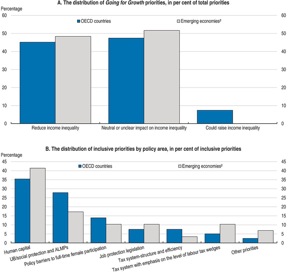
← 1. Going for Growth priorities are considered as inclusive when associated recommendations are likely to reduce income inequality. They are considered as neutral in terms of inclusiveness when their impact on income inequality is either unknown or null. Finally, priorities are considered as adverse for inclusiveness when associated recommendations may trigger an increase in income inequality. See text and also Chapter 1.
2. Emerging economies include non-OECD countries (Argentina, Brazil, China, Colombia, Costa Rica, India, Indonesia, Lithuania and South Africa) along with Chile, Mexico and Turkey.
29. Against this background, Going for Growth focuses on the following major policy areas where actions have the largest scope to make growth more inclusive:
-
Education policies: focusing on the early years, on the needs of families with school children, and on providing youth with the skills they need to get a good start in the labour market;
-
Skills and training: encouraging a continuous up-grading of skills during the working life in order to adapt to a rapidly evolving economy;
-
Labour market policies: promoting access to jobs (and job formalisation for emerging economies) as well as labour market integration of under-represented groups in order to raise job quantity and quality;
-
Tax and transfer systems:30 designing taxes and transfers to achieve growth-friendly and cost-effective redistribution, that is to contain inequality without undermining incentives to work and invest, including through in-kind public transfers (e.g. public provision of health and education services).
30. The discussion in this section is structured on the basis of common inclusiveness challenges that countries can address with a relevant package of policy reforms in the above identified areas. It focuses on three broad challenges: i) skills and equity in education, ii) labour market insecurity and segmentation and, iii) the gender gap and women’s integration in economic activities. Such challenges are not meant to be exhaustive, which largely reflects the granularity of countries’ situations. Associated policy reform recommendations are detailed in the country notes (see Chapter 3).
Skills and equity in education
31. Improving outcomes and equity in education and skills is fundamental to boost growth and make it more inclusive. Education shapes each individual’s life chances and is closely related to skills and training which in turn determines people’s ability to earn a decent living. Progress in this area can make growth more inclusive through a number of channels, in particular by:
-
Enhancing equality of opportunities hence intergenerational social mobility, which in turn improves the allocation of talents and human capital and ultimately economic growth;
-
Enhancing employment prospects, including chances of formal employment in emerging economies, and securing adaptability of the workforce to changing demand for skills, all of which are important prerequisites for economic growth;
-
Broadening the base for productivity growth to make it more inclusive and ensure that it benefits wider parts of society. In this respect, education and training are key remedies to combat the twin challenge of slowing productivity growth and rising inequality faced by many OECD countries (OECD, 2016a; 2016b);
-
Contributing to greater well-being through several non-income dimensions, many of which features in the OECD Better Life Index (OECD, 2015d). For instance, life expectancy tends to be closely related to educational level (OECD, 2015e) and education has been found to have favourable effects on health status, crime and civic engagement.31
32. Education has a special policy traction for emerging economies to achieve convergence in living standards vis-à-vis advanced economies, while ensuring that growth dividends contribute to the expansion of the middle class. The share of the population with at least upper-secondary education is still well below the OECD average in most emerging economies (Figure 2.9), even though substantial improvements have taken place. For instance in Latin American countries, the share of 25-34 year-olds with at least upper-secondary education exceeds the share for the total population by 10-20 percentage points.
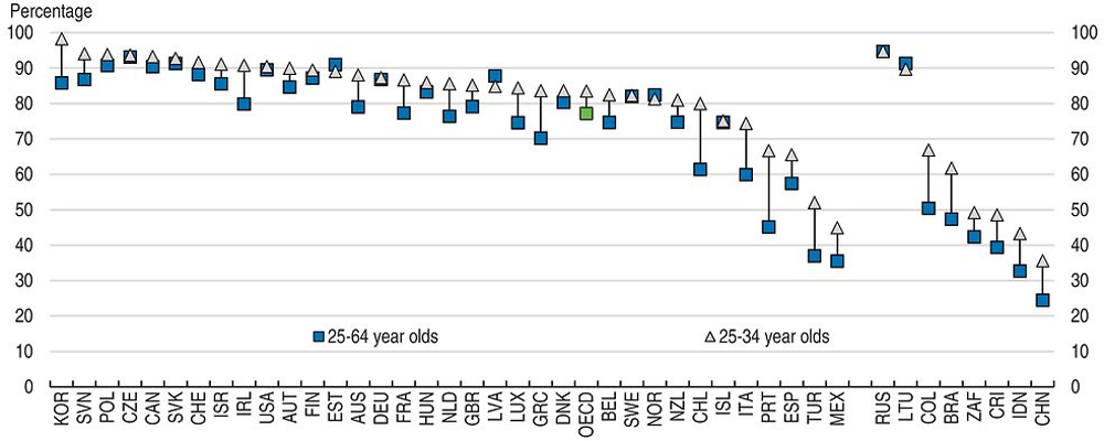
← 1. Data refer to 2010 for China; 2013 for Indonesia and the Russian Federation; 2014 for Brazil and South Africa.
Source: OECD, Education at a Glance 2016: OECD Indicators.
33. Educational inequalities are deeply related to regional inequalities, notably in China and India, reflecting inequalities of opportunities in access to education (as well as other public services such as healthcare) between rural and urban areas. Educational inequalities are also related to gender inequalities, for instance in terms of secondary education enrolment gaps. Equal access to education in emerging economies is still hampered by financial constraints as well as lack of infrastructure. However, the critical obstacle to catch-up with respect to high-income countries, both in terms of growth and equity, is in most cases the low quality of schooling.32 As a result, educational outcomes are far below the OECD average and strongly linked to socio-economic background (OECD, 2012a).
34. Educational inequalities start early and disadvantages cumulate over the lifecycle. Children of parents with high education levels and high incomes generally have a much higher chance of performing well compared to children from more disadvantaged families.33 Neighbourhood effects, socio-economic segregation across schools and unequal access to quality teaching by students who would gain most from it have also been found to have a significant impact on educational opportunities, hence on social mobility.34 The strong impact of social background on students’ outcomes is evident in results from PISA, not only the impact of own social background on individual outcomes, but also the impact of school social background (that is, the average social background of students within a given school) on individual outcomes. These effects are exacerbated for children of migrants, which tend to be socio-economically disadvantaged and display a large performance gap with respect to non-immigrant students (OECD, 2013a).
35. The case for enhancing equity in education is strong and widespread, but the estimated relationship between students’ performance and socio-economic background varies substantially across countries and some, such as Estonia and Japan, combine strong performance in science with strong equity (Figure 2.10). This suggests that some countries and some education systems do a better job of minimising the impact of social differences in education; which does not come at the expense of lower overall performance, quite the contrary if anything.
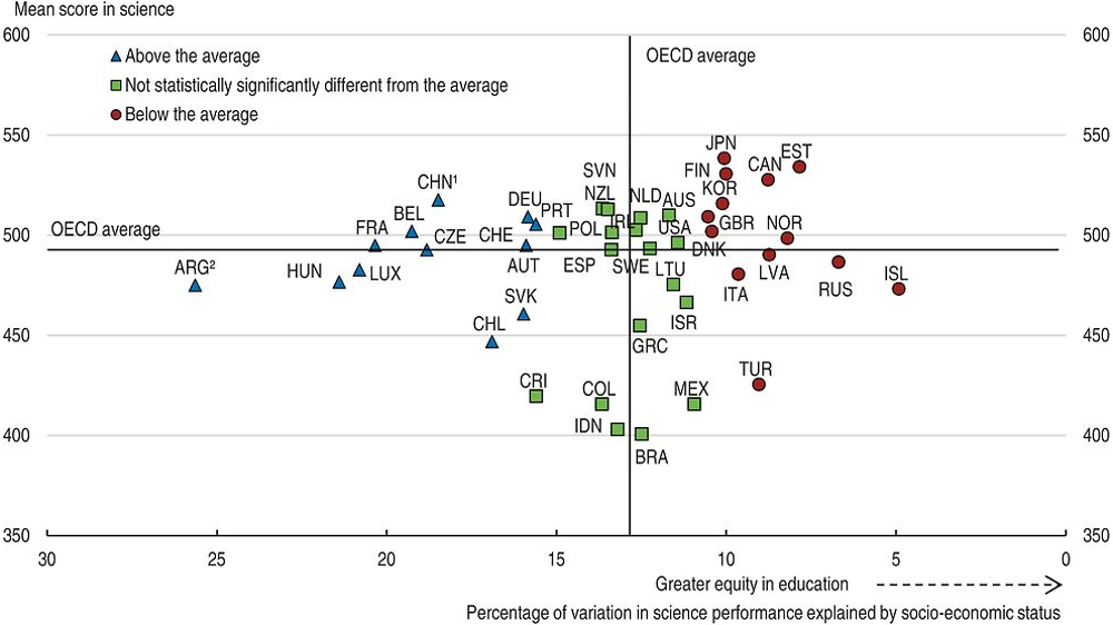
1. Data refer to the four PISA participating Chinese provinces: Beijing, Shanghai, Jiangsu and Guangdong.
2. Data refer to the region of Ciudad Autonoma de Buenos Aires. Coverage is too small to ensure comparability (see Annex A4 of PISA 2015 Results, Volume I: Excellence and Equity in Education).
Source: OECD (2016), PISA 2015 Results (Volume I): Excellence and Equity in Education.
36. Inequality in skills translates into inequality in incomes, starting with market incomes. Wage dispersion has been a strong driver of rising inequality over the last decades. This has been notably driven by skill-biased technological change while upskilling has had a mitigating effect. Recent evidence points to increased computerisation of routine tasks contributing to the erosion of many middle-income jobs hence to the rise in job polarisation.35 In this context, the types of skills workers acquire and their proficiency in these skills have become at least as important as their formal level of education. Differences in skills have for instance been found to account for a substantial part of the wage gap between native and foreign-born workers and around one-fifth of the wage gap between men and women (OECD, 2015c, Chapter 2).
37. Mismatches between the qualifications and skills of workers and demands of employers prevail in many OECD countries (Figure 2.11), with over-skilling, and thus earnings below potential, being the main issue (Adalet McGowan and Andrews, 2015). Skill mismatches are widespread in countries such as Italy, Spain and the Czech Republic, while in other countries such as France and the United Kingdom under skilling is a particular challenge. Recent evidence suggests that wage inequality is lower in countries that are better at meeting the demand for skills, especially in the upper half of the wage distributions (OECD, 2015c, Chapter 2). More efficient allocation of labour resources may thus both raise labour productivity and reduce earnings inequality.
38. Enhancing equity in education and skills requires reforms in a broad range of policy areas, from pre-school to university, as well as school-to-work transition, training and life-long learning. In this respect, investing in early childhood education and care has been shown to yield some of the largest returns because a person can build on the acquired learning as input in later education stages, resulting in a process of dynamic synergies.36 Returns from early intervention are particularly high for children from disadvantaged backgrounds, including children of migrants and refugees with language difficulties. Access to affordable childcare and pre-schools are thus strong instruments to ensure equity in compulsory education.
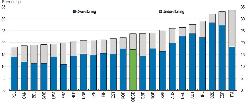
← 1. Based on OECD calculations using OECD Survey of Adult Skills (2012). The OECD average is the unweighted average for available countries.
Source: Adalet McGowan, M. and D. Andrews (2015), “Skill Mismatch and Public Policy in OECD Countries”, OECD Economics Department Working Papers, No. 1210.
39. Striving for equity in higher education is less obvious. Publicly-financed access to higher education (either direct or via subsidies, including via student grants) may overcome credit constraints and favour equality of opportunity. At the same time, tertiary graduation is an investment in human capital, which paves the way for a relatively high lifetime income, thereby weakening the equity argument for tax-financed higher educational services (to the extent that part of the funding comes from lower educated individuals who do not benefit from associated services).37 From a policy perspective, tuition fees combined with financial support (i.e. mean-tested grants and income-contingent payback loans) for students from least well-off families are considered to achieve the best balance between growth and equity objectives (Wössmann, 2008).
40. While the potential returns from educational and skill reforms are large, their effects are likely to take time to materialise. Raising the level of educational attainment in the workforce takes time and higher social mobility takes at least a generation for the full effects to unfold. However, the case for emphasising education and skill reforms remains very strong. Progress in this area is a form of ex ante redistribution because it improves equality in market incomes. This may reduce the need and scope for governments’ ex post redistribution, that is, through taxes and transfers.38 Provision of public education can in this respect be considered as a more active approach to redistribution, taking into account equity and efficiency considerations.39
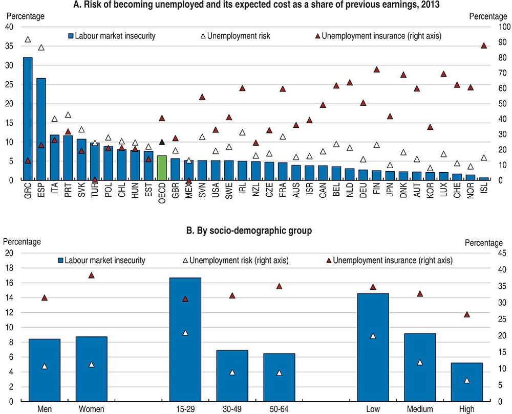
← 1. Labour market insecurity (%) is defined in terms of the expected earnings loss associated with unemployment. This loss depends on the risk of becoming unemployed, the expected duration of unemployment and the degree of mitigation against these losses provided by government transfers to the unemployed (effective insurance). Unemployment risk (%) is measured as the monthly unemployment inflow probability times the expected average duration of unemployment spells (in months). Unemployment inflow probability is the ratio of unemployed persons who have been unemployed for less than one month over the number of employed persons one month before. Unemployment insurance (%) is defined as the coverage rate of unemployment insurance (UI) times its average net replacement rate among UI recipients plus the coverage rate of unemployment assistance (UA) times its net average replacement rate among UA recipients. The average replacement rates for recipients of UI and UA take account of family benefits, social assistance and housing benefits. In Panel A the data for Chile refer to 2011 instead of 2013.
Source: OECD, Job Quality Database.
Labour market insecurity and segmentation
41. Labour market insecurity has special policy traction from an inclusive growth perspective because it is broadly defined, encompassing both job quantity and job quality. Labour market insecurity captures those aspects of economic insecurity that are related to the probability of job loss (unemployment risk), the duration of unemployment and the economic cost for workers (unemployment insurance, Figure 2.12, Panel A).40 Youth and the low-skilled face considerably higher labour market insecurity than other socio-demographic groups (Figure 2.12, Panel B), in addition to having the poorest performance in terms of employment and unemployment. This reflects to a large extent their overrepresentation among non-regular employees, facing higher risk of job loss and less social protection in the event of job loss (OECD, 2014b, Chapter 4). Moreover, evidence suggests that non-regular contracts are rarely a stepping stone into stable employment and therefore that associated inequalities relative to regular contracts tend to persist over time. Labour market insecurity and labour market segmentation are therefore closely linked, by affecting disproportionality certain categories of workers.
42. In emerging economies, labour market insecurity also covers informality and the risk of extreme low pay. In most of these countries, the main challenge is not a lack of jobs since open unemployment tends to be relatively low. High levels of labour market insecurity are generally driven by high risks of extreme low pay, rather than by high unemployment, with the exception of South Africa (Figure 2.13, Panel A). Such risk is concentrated among informal workers, as evidence suggests that informality is hard to escape and starting a career with an informal job may have negative consequences for future labour market prospects (Figure 2.13, Panel B).
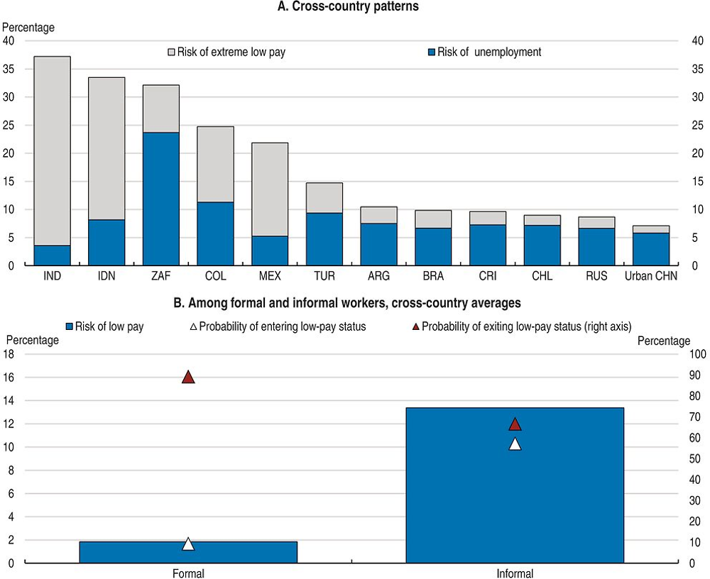
← 1. In the first Panel, overall labour market insecurity is calculated as insecurity from unemployment plus the insecurity from extreme low pay if employed. The divide between formal and informal status is based on social security payments (employees) and business registration (self-employed), except for Colombia and the Russian Federation where information on work contract (written or not) was used.
Source: OECD (2015), OECD Employment Outlook 2015.
43. Reducing labour market insecurity and its disproportionate incidence on youth, low-skilled and informal workers has the potential to boost growth by enhancing labour market reallocation and can make growth more inclusive through several channels, in particular by:
-
Reducing unemployment incidence and duration, hence income inequality between workers and non-workers;
-
Reducing labour market dualism, hence unequal access to social protection and training between regular (formal) and non-regular (informal) workers, and therefore earnings as well as disposable income inequality;
-
Enhancing career prospects over the lifecycle, hence reducing inequality from a dynamic perspective and spurring social mobility.
44. Reducing labour market insecurity would not only promote growth and make it more inclusive but also, going beyond, improve well-being. Indeed, new evidence suggests that the well-documented detrimental effect of unemployment on individual well-being is to a large extent a reflection of the risk of staying unemployed for a prolonged period of time (Hijzen and Menyhert, 2016). This implies that policy makers should focus not only on reducing the level of unemployment but also on speeding up the return to work, providing thus an additional rationale for combating long-term unemployment in countries where its incidence is relatively high, such as in Continental and Southern European, as well as in countries where it has increased significantly, such as the United States.
45. From an inclusiveness perspective, addressing labour market insecurity is a particularly pressing challenge in the case of European Mediterranean countries (Greece, Italy, Portugal and Spain, Figure 2.12), reflecting its high level and adverse trend, exacerbating the risk of social exclusion today and potentially weighing on equity and growth outcomes tomorrow. These countries were hard hit by the crisis. The recession and slow recovery have contributed to increase poverty risk and depth (Figure 2.7), both of which were already comparatively high before the crisis. Among vulnerable groups, youth stand out as having borne a disproportionate share of the burden of high joblessness since 2007. Youth unemployment has been falling since the recovery but in European Mediterranean countries it remains extremely high, above 30% (OECD, 2016d, Chapter 1). The exclusion of youth from the labour market undermines long-run growth through skills erosion and reduces the prospect of career building and social mobility, with the risk of a further widening of inequality.
46. The broad picture of youth vulnerability is reinforced by looking at NEET status which is more closely connected to the risk of long-run marginalisation in the labour market than youth unemployment. Again, in European Mediterranean countries hit hardest by the crisis a particularly high and rising share of young people is NEET, but the challenge goes well beyond this group of countries. High NEET levels are also observed in some of the countries enjoying among the highest educational outcomes in the OECD such as Korea and France (Figure 2.14). Recent analysis shows that slightly more than one-third of 15-29 year-old NEETs live in a jobless household, across OECD countries for which data are available. This share rises to 44% for low‐skilled NEETs, suggesting that many in this group experience both low current incomes and high risk of poverty in the short-run as well as limited career opportunities in the long run. The United Kingdom exhibits the highest share of low-skilled NEET living in a jobless household, i.e. 60%, compared to less than 10% of other youth. For this generation, the longer the time that is spent out of work and out of training, the higher the risk of potential long-term and long-lasting negative effects on labour market outcomes and, more broadly, higher risks of social exclusion.41
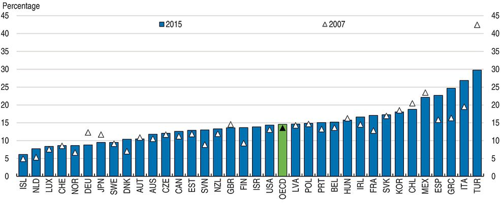
← 1. For 2007, data is not available for Israel; 2006 for Chile. The last available year is 2013 for Chile and Korea and 2014 for Israel.
Source: OECD (2016), OECD Employment Outlook 2016.
47. Achieving a balanced approach between, on the one hand, boosting job quantity and quality by raising labour supply and demand incentives and, on the other hand, ensuring income adequacy across individuals and throughout the lifecycle, requires policy reforms in a number of areas – as widely documented over the years in the vast policy-oriented research on labour markets and social policies – such as:42 i) labour market policies, including job protection legislation, ALMPs and minimum wages; ii) skills and training policies, including VET and apprenticeships systems; iii) taxes and transfers, including employment-related, universal and means-tested social transfers, as well as labour tax wedges at low incomes with an increasing emphasis on earned income tax credits (EITC).
48. In the pursuit of labour market inclusiveness, governments need to enhance migrants’ integration in the labour market. Labour market integration is key to achieve migrants’ integration in society at large and would help reducing their high and rising poverty risks.43 In this respect, lowering barriers to “employability” is essential for migrants’ ability to get a regular job, which requires better recognition of skills acquired abroad and expansion of language courses; as well as ALMPs and coaching to address potential information hurdles beyond language barriers. Achieving progress in this area is becoming all the more pressing in light of recent and future trends in migrants’ inflows, especially in the context of the refugee crisis in Europe (European Commission, 2016).
49. Addressing labour market insecurity is a challenge for all emerging economies and this requires reducing informality, given the strong association between informality and labour market insecurity. Beyond such broad challenge, the situation differs greatly across countries, not only reflecting the incidence but also the nature of informal work. One worrying fact is that countries exhibiting the highest share of informal workers, e.g. Indonesia, India, and Mexico, have not registered much improvement over the latest period, based on available estimates (OECD, 2015c, Chapter 5). Still, despite the progress achieved in a number of other emerging economies, more needs to be done to reduce informality. Countries share a common set of broad reform recommendations in this area, in particular developing adequate and effective social protection systems as well as ALMPs, simplifying and enhancing the effectiveness of labour market regulations and institutions (including their enforcement), and reducing the costs of formalisation for firms, i.e. low-skilled employment costs and administrative burdens to entrepreneurship.
The gender gap and the integration of women in economic activities
50. Overcoming gender inequalities is fundamental to achieve inclusive growth, contributing not only to raise equity but also to improve efficiency. The social and equity arguments for enhancing the integration of women in the labour market and, more broadly, in economic activities, are strong and multiple, in particular in terms of:
-
Reducing income inequality, as evidence suggests that progress in this area over the last two decades has limited the rise in inequality. If the proportion of households with working women had remained at levels of 20 to 25 years ago, income inequality would have increased by almost 1 point more on average on the Gini coefficient scale. The impact of a higher share of women working full-time and higher relative wages for women slowed the rise of inequality by one 1 additional point (OECD, 2015b, Chapter 5).
-
Reducing poverty risk and in particular child poverty, as families where no-one is working and single mothers are more likely to fall below the poverty line, and children living in such families may face a lifetime of disadvantage. Such argument is particularly relevant for emerging economies, reflecting the prevalence of still large gender gaps as well as material deprivation among children. Across OECD countries for which comparable data are available, Israel and Turkey suffer from the highest child poverty rates and this is associated with large gender gaps (see Table 2.A1.1 in the Annex).44
-
Reducing dualism by enhancing women inclusion in the labour market, in particular in countries exhibiting large gender gaps and overrepresentation of women among non-regular workers, as is the case in Japan and Korea (OECD, 2014b, Chapter 4).
-
Reducing old-age poverty risk: indeed, while old-age poverty has declined dramatically across OECD countries over the last decades, there remains a clear gender gap as women face substantially higher risk of poverty than their male counterparts.45 For example, in the United States, the poverty rate among older men is around 16.5% while it rises to 25.6% for women. In Germany and Finland, where poverty is much lower than the United States, the risk is however two times higher for older women compared to older men (OECD, 2015g). This pattern can arise from substantial gaps in pensions which in turn reflect gender gaps in remuneration, working hours and duration of working lives, in particular women’s interrupted working lives.
51. Progress has been achieved in this area, as employment and wage gaps between men and women have been narrowing across many countries. Over the last decade the employment gap has narrowed by 4 percentage points on average across the OECD (Figure 2.15, Panel A). However this gap still stands at 11 points, and widens to close to 22 points by taking into account the fact that more women work part time than men (OECD, 2015b, Chapter 5). In addition, the average gender gap masks substantial cross-country heterogeneity: for instance the gender wage gap (unadjusted for occupational and qualification differences) ranges from above 25% in Korea and Japan to below 5% in Belgium and Luxembourg (Figure 2.15, Panel B).
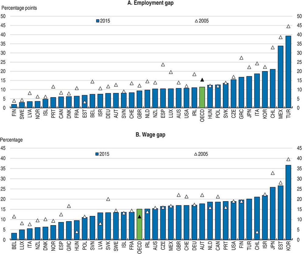
← 1. The employment gap is defined as the difference between male and female employment rates for 15-64 year-olds. The wage gap is defined as the difference between median wages of men and women, expressed in per cent of median wages for men. Estimates of earnings refer to gross earnings of full-time wage and salary workers. Both gaps are unadjusted in the sense that they do not take into account personal characteristics such as education and work experience. For Panel B data for 2015 refer to 2010 for Estonia, Latvia, Luxembourg, the Netherlands, Slovenia and Turkey; 2011 for Israel; 2012 for France and Spain; 2013 for Sweden; and 2014 for Australia, Austria, Belgium, Denmark, Finland, Germany, Greece, Iceland, Ireland, Italy, Japan, Korea, New Zealand, Poland, Portugal and Switzerland. Data for 2005 refer to 2006 for Chile, Estonia, Italy, Latvia, Luxembourg, the Netherlands, Poland and Switzerland; 2008 for Denmark. Data from mid-2000s are not available for Slovenia and Turkey.
Source: OECD, Labour Force Statistics and Earnings Inequality Databases.
52. OECD countries have been increasingly responsive to the challenge of tackling gender gaps, as testified by the acceleration of policy reforms to remove barriers to full-time (as well as voluntary part-time) labour market participation of women (see Chapter 3). Despite the progress achieved, the challenge remains and is widely spread, as more needs to be done to enhance the inclusion of women in the labour market.46 This requires policy reforms in a number of areas, and the provision of quality childcare and early childhood policies is key in this respect. Progress along these lines is fundamental not only to allow women to better combine family and work responsibilities, but also to promote equality of educational opportunities for children from disadvantaged backgrounds. Many OECD countries need also pursuing tax and transfer reforms to remove fiscal disincentives for women to participate in the labour market at their full potential. Reforms in this area would improve horizontal inclusiveness in the tax system, i.e. its neutrality towards taxpayers regardless of their gender.47
53. Empowering women in society is a challenge among all emerging economies, not least because gender gaps are generally higher than among advanced economies. Reducing those gaps would not only reduce income inequality and enhance inclusiveness, but also, importantly, curb child poverty and malnutrition because women account for the majority of primary-care givers. Recent analysis suggests that closing gender gaps in the labour markets of emerging economies is still an unfinished job (OECD, 2016c, Chapter 4):
-
The gender gap in labour market participation is shrinking in many emerging economies, but progress has been very uneven. The most significant improvements have been recorded in Latin America, particularly in Chile and Costa Rica, while larger gaps persist in countries such as India and Indonesia.
-
The share of NEET is higher among women than men, partly reflecting motherhood at a young age in some emerging economies, especially in India but also in Turkey and Mexico.
-
Female workers in emerging economies continue to have worse jobs than men, for example because employed women are overrepresented in low productivity and low pay sectors; and self-employed women are overrepresented in low profitability businesses as well as in informal jobs. As a result, women have less secure jobs than men, facing both a higher unemployment risk and a higher risk of extreme low pay, as emphasised above.
-
Closing gender gaps in emerging economies requires concerted action across a broad spectrum of policy domains, with an emphasis on tackling the remaining gaps in education and access to capital; but also, as in advanced countries, freeing women’s time by, for example, expanding subsidised childcare and promoting flexible employment; as well as addressing fiscal disincentives and other regulations that limit female participation in the formal labour market; and, last but not least, fighting gender discrimination and violence against women.
References
Adalet McGowan, M. and D. Andrews (2015), “Labour Market Mismatch and Labour Productivity: Evidence from PIAAC Data”, OECD Economics Department Working Paper, No. 1209, OECD Publishing, Paris, https://doi.org/10.1787/5js1pzx1r2kb-en.
Aghion, P. et al. (2016), “Living the ’American Dream’ in Finland: The Social Mobility of Inventors”, mimeo.
Aghion, P. et al. (2015), “Innovation and Top Income Inequality”, NBER Working Paper, No. 21247.
Altzinger, W. et al. (2015), “Education and Social Mobility in Europe: Levelling the Playing Field for Europe’s Children and Fuelling its Economy”, WWWforEurope Working Paper, No. 80.
Arntz, M., T. Gregory and U. Zierahn (2016), “The Risk of Automation for Jobs in OECD Countries: A Comparative Analysis”, OECD Social, Employment and Migration Working Papers, No. 189, OECD Publishing, Paris, https://doi.org/10.1787/5jlz9h56dvq7-en.
Atkinson, A.B. (2015), Inequality: What can be done?, Harvard University Press.
Atkinson, A.B. (1970), “On the Measurement of Inequality”, Journal of Economic Theory, Vol. 2, pp. 244-263.
Autor, D.H., F. Levy and R.J. Murnana (2003), “The Skill Content of Recent Technological Change: An Empirical Exploration”, Quarterly Journal of Economics, Vol. 118/4, pp. 1279-1333.
Bjorklund, A. and K.G. Salvanes (2011), “Education and Family Background: Mechanisms and Policies”, in E.A. Hanushek, S. Machin and L. Woessmann (eds.), Handbook of the Economics of Education, Vol. 3, pp. 201-247.
Braconier, H. and J. Ruiz Valenzuela (2014), “Gross Earning Inequalities in OECD Countries and Major Non-member Economies: Determinants and Future Scenarios”, OECD Economics Department Working Papers, No. 1139, OECD Publishing, Paris, https://doi.org/10.1787/5jz123k7s8bv-en.
Brys, B. et al. (2016), “Tax Design for Inclusive Economic Growth”, OECD Taxation Working Papers, No. 26, OECD Publishing, Paris, https://doi.org/10.1787/5jlv74ggk0g7-en.
Causa, O., M. Hermansen and N. Ruiz (2016), “The Distributional Impact of Structural Reforms”, OECD Economics Department Working Papers, No. 1342, OECD Publishing, Paris, https://doi.org/10.1787/5jln041nkpwc-en.
Causa, O., A. de Serres and N. Ruiz (2015), “Can pro-growth policies lift all boats? An analysis based on household disposable income”, OECD Journal: Economic Studies, Vol. 2015/1, OECD Publishing, Paris, https://doi.org/10.1787/eco_studies-2015-5jrqhbb1t5jb.
Causa, O. and A. Johansson (2009), “Intergenerational Social Mobility”, OECD Economics Department Working Papers, No. 707, OECD Publishing, Paris, https://doi.org/10.1787/223106258208.
Chetty, R., N. Hendren and L.F. Katz (2016), “The Effects of Exposure to Better Neighborhoods on Children: New Evidence from the Moving to Opportunity Experiment”, American Economic Review, Vol. 106/4, pp. 855-902.
Cournède, B., O. Denk and P. Garda (2016), “Effects of Flexibility-Enhancing Reforms on Employment Transitions”, OECD Economics Department Working Papers, No. 1348, OECD Publishing, Paris, https://doi.org/10.1787/bd8e4c1f-en.
Deaton, A. (1997), The Analysis of Household Surveys, Johns Hopkins University Press.
European Commission (2016), “An Economic Take on the Refugee Crisis: A Macroeconomic Assessment for the EU”, Institutional Paper, No. 33.
Fournier, J.M. and I. Koske (2012), “The Determinants of Earnings Inequality: Evidence from Quantile Regressions”, OECD Journal: Economic Studies, Vol. 2012/1, pp. 7-36, https://doi.org/10.1787/eco_studies-2012-5k8zs3twbrd8.
Gal, P. and A. Theising (2015), “The Macroeconomic Impact of Structural Policies on Labour Market Outcomes in OECD Countries: A Reassessment”, OECD Economics Department Working Papers, No. 1271, OECD Publishing, Paris, https://doi.org/10.1787/5jrqc6t8ktjf-en.
Galor, O. and J. Zeira (1993), “Income Distribution and Macroeconomics”, Review of Economic Studies, Vol. 60/1, pp. 35-52.
Geppert, C. and M. Lüske (2017), “ Labour Supply Effects of Pension Policies and Early Retirement Schemes: Differences across Socio-Economic Groups”, OECD Social, Employment and Migration Working Papers, forthcoming, OECD Publishing, Paris.
Glewwe, P. and K. Muralidharan (2016), “Improving Education Outcomes in Developing Countries: Evidence, Knowledge Gaps, and Policy Implications”, in E.A. Hanushek, S. Machin and L. Woessmann (eds.), Handbook of the Economics of Education, Vol. 5, pp. 653-743.
Hacker, J. (2011), “The Institutional Foundations of Middle Class Democracy”, Policy Network, essay.
Haitz, N. (2015), “Old-age Poverty in OECD Countries and the Issue of Gender Pension Gaps”, CESifo DICE Report, Vol. 13/2, pp. 73-75.
Heckman, J.J. and S. Mosso (2014), “The Economics of Human Development and Social Mobility”, Annual Review of Economics, Vol. 6, pp. 689-733.
Hermansen, M., N. Ruiz and O. Causa (2016), “The Distribution of the Growth Dividends”, OECD Economics Department Working Papers, No. 1343, OECD Publishing, Paris, https://doi.org/10.1787/7c8c6cc1-en
Hijzen, A. and B. Menyhert (2016), “Measuring Labour Market Security and Assessing its Implications for Individual Well-Being”, OECD Social, Employment and Migration Working Papers, No. 175, OECD Publishing, Paris, https://doi.org/10.1787/5jm58qvzd6s4-en.
Immervoll, H. and L. Richardson (2011), “Redistribution Policy and Inequality Reduction in OECD Countries: What Has Changed in Two Decades?”, OECD Social, Employment and Migration Working Papers, No. 122, OECD Publishing, Paris, https://doi.org/10.1787/5kg5dlkhjq0x-en.
Knight, J. and R. Sabot (1983), “Educational Expansion and the Kuznets Effects”, American Economic Review, Vol. 73/5, pp. 1132-1136.
Lochner, L. (2011), “Nonproduction Benefits of Education: Crime, Health, and Good Citizenship”, in E.A. Hanushek, S. Machin and L. Woessmann, Handbook of the Economics of Education, Vol. 4, pp. 183-282.
Marlier, E. and A.B. Atkinson (2010), “Indicators of Poverty and Social Exclusion in a Global Context”, Journal of Policy Analysis and Management, Vol. 29, pp. 285-304.
Marx, I., B. Nolan and J. Olivera (2015), “The Welfare State and Antipoverty Policy in Rich Countries”, in A.B. Atkinson and F. Bourguignon (eds.), Handbook of Income Distribution, Vol. 2B, North-Holland, pp. 2063-2139.
Michaels, G., A. Natraj and J. Van Reenen (2014), “Has ICT Polarized Skill Demand? Evidence from Eleven Countries over Twenty-Five Years”, Review of Economics and Statistics, Vol. 96/1, pp. 60- 77.
Murtin, F. and A. de Serres (2014), “How Do Policies Affect the Exit Rate out of Unemployment? Disentangling Job Creation from Labour Market Frictions”, LABOUR, Vol. 28/2, pp. 190-208.
OECD (2016a), The Productivity-Inclusiveness Nexus, Meeting of the OECD Council at Ministerial Level, www.oecd.org/mcm/documents/The-productivity-inclusiveness-nexus.pdf.
OECD (2016b), OECD Economic Outlook, Volume 2016 Issue 1, OECD Publishing, Paris, https://doi.org/10.1787/eco_outlook-v2016-1-en.
OECD (2016c), OECD Employment Outlook 2016, OECD Publishing, Paris https://doi.org/10.1787/empl_outlook-2016-en.
OECD (2016d), OECD Economic Surveys: Korea 2016, OECD Publishing, Paris. https://doi.org/10.1787/eco_surveys-kor-2016-en.
OECD (2016e), Education at a Glance 2016: OECD Indicators, OECD Publishing, Paris, https://doi.org/10.1787/eag-2016-en.
OECD (2016f): PISA 2015 Results (Volume I): Excellence and Equity in Education, OECD Publishing, Paris, https://doi.org/10.1787/9789264266490-en.
OECD (2015a), Economic Policy Reforms 2015: Going for Growth, OECD Publishing, Paris https://doi.org/10.1787/growth-2015-en.
OECD (2015b), In It Together: Why Less Inequality Benefits All, OECD Publishing, https://doi.org/10.1787/9789264235120-en.
OECD (2015c), OECD Employment Outlook 2015, OECD Publishing, Paris, https://doi.org/10.1787/empl_outlook-2015-en.
OECD (2015d): How’s Life? 2015: Measuring Well-being, OECD Publishing, Paris, https://doi.org/10.1787/how_life-2015-en.
OECD (2015e), Health at a Glance 2015: OECD Indicators, OECD Publishing, Paris, https://doi.org/10.1787/health_glance-2015-en.
OECD (2015f), International Migration Outlook 2015, OECD Publishing, Paris, https://doi.org/10.1787/migr_outlook-2015-en.
OECD (2015g), Pensions at a Glance 2015: OECD and G20 indicators, OECD Publishing, Paris, https://doi.org/10.1787/pension_glance-2015-en.
OECD (2014a), All on Board: Making Inclusive Growth Happen, OECD Publishing, Paris, https://doi.org/10.1787/9789264218512-en.
OECD (2014b), OECD Employment Outlook 2014, OECD Publishing, Paris, https://doi.org/10.1787/empl_outlook-2014-en.
OECD (2013a), PISA 2012 Results: Excellence through Equity (Volume II): Giving Every Student the Chance to Succeed, OECD Publishing, Paris, https://doi.org/10.1787/9789264201132-en.
OECD (2013b), Recommendation of the Council on Gender Equality in Education, Employment, and Entrepreneurship, OECD Publishing, Paris, www.oecd.org/gender/C-MIN(2013)5-ENG.pdf.
OECD (2012a), Low-Performing Students: Why They Fall Behind and How to Help Them Succeed, OECD Publishing, Paris, https://doi.org/10.1787/9789264250246-en.
OECD (2012b), Starting Strong III: A Quality Toolbox for Early Childhood Education and Care, OECD Publishing, Paris, https://doi.org/10.1787/9789264123564-en.
OECD (2011a), Divided We Stand: Why Inequality Keeps Rising, OECD Publishing, https://doi.org/10.1787/9789264119536-en.
OECD (2011b), How’s Life?: Measuring Well-being, OECD Publishing, Paris, https://doi.org/10.1787/9789264121164-en.
OECD (2008), Growing Unequal?: Income Distribution and Poverty in OECD Countries, OECD Publishing, Paris, https://doi.org/10.1787/9789264044197-en.
OECD/Korea Institute of Public Finance (2014), The Distributional Effects of Consumption Taxes in OECD Countries, OECD Publishing, Paris, https://doi.org/10.1787/9789264224520-en.
Piketty (2013), Le Capital au XXI e siècle, Éditions du Seuil, Paris.
Ravallion, M. (2012), “Why Don’t We See Poverty Convergence?”, American Economic Review, Vol. 102/1, pp. 504-523.
Ruiz, N. and N. Woloszko (2015), “What Do Household Surveys Suggest about the Top 1% Incomes and Inequality in OECD Countries?”, OECD Economics Department Working Papers, No. 1265, OECD Publishing, Paris, https://doi.org/10.1787/5jrs556f36zt-en.
Sen, A. (1999), Development as Freedom, Oxford University Press.
Voitchovsky, S. (2005), “Does the Profile of Income Inequality Matter for Economic Growth?”, Journal of Economic Growth, Vol. 10, pp. 273-296.
World Bank (2016), Taking on Inequality: Poverty and Shared Prosperity 2016, World Bank Group.
World Bank (2015), “A Measured Approach to Ending Poverty and Boosting Shared Prosperity: Concepts, Data, and the Twin Goals”, Policy Research Report, World Bank.
Wössmann, L. (2008), “Efficiency and Equity of European Education and Training Policies”, International Tax and Public Finance, Vol. 15, pp. 199-230.
Notes
← 1. The statistical data for Israel are supplied by and under the responsibility of the relevant Israeli authorities. The use of such data by the OECD is without prejudice to the status of the Golan Heights, East Jerusalem and Israeli settlements in the West Bank under the terms of international law.
← 2. Successive issues of Going for Growth have already emphasised that while rising GDP per capita has certainly the potential to make all citizens better off materially, evidence shows that the benefits of growth need not benefit all across the income distribution (OECD, 2015a). The extension of the framework is in line with some of the key recommendations put forward by the Commission on the Measurement of Economic Performance and Social Progress and followed up in the OECD Better Life Initiative and the OECD Inclusive Growth framework (OECD, 2014a).
← 3. Higher household disposable income may not necessarily bring improvements in other aspects of well-being such as participation in productive activities, education and good health. Income is arguably the most important contributor to well-being, but non-income dimensions also matter (OECD, 2014a).
← 4. See OECD (2014b, Chapter 3; 2015c, Chapter 5) for details and references. The OECD Job Quality framework also includes one additional dimension not considered here, that is, the quality of the working environment. This captures non-economic aspects of job quality and includes factors that relate to the nature and content of work performed, working-time arrangements and workplace relationships. The reason for not yet incorporating the quality of working environment in the current Going for Growth extension relates to data availability issues as well as to the still relatively limited evidence on the impact of pro-growth policies on such dimension of job quality and, more broadly, well-being.
← 5. Available measures with a sufficiently broad time and country coverage – generallybased on variants of life expectancy – remain relatively poor proxies of health outcomes and further statistical progress is needed in this area.
← 6. For example, the next edition of the OECD Better Life Index is planned to include a broader range of inequality dimensions which could be taken on board in future editions of Going for Growth.
← 7. The focus of such quantitative assessment is on long-term effects, in line with the broad orientation of Going for Growth, i.e. boosting long-term living standards. At the same time, short-term and country-specific imperatives are ultimately taken into account when formulating a relevant package of policy recommendations via the qualitative assessment, based on consultation with country experts.
← 8. See Immervoll and Richardson (2011) on redistribution policy and inequality reduction in OECD countries.
← 9. Research on the policy drivers of poverty is abundant for developing countries. The World Bank produces a substantive amount of policy-relevant work in this area which can be relied upon for assessing reform recommendations for emerging economies (World Bank, 2015). However, much less is available in the case of high-income countries on the policy drivers of poverty risk and depth. The matching and example above relies on evidence summarised in the Handbook for Income Distribution (Marx et al., 2015).
← 10. Another strong argument in this respect is recent empirical evidence on the distributional effect of economic growth: Hermansen et al. (2016) show that employment-rich growth reducesincome inequalities by boosting incomes in the middle class and among the poor.
← 11. See also OECD (2016c), Chapter 3, for a discussion on policy packages to mitigate potential short-term employment and wage losses associated with reforms that reduce barriers to entry in product markets and reforms that increase flexibility in regulation governing the dismissal of workers on regular contracts.
← 12. That is the case in a static perspective as opposed to over the lifecycle, in which case the effect comes closer to being distribution-neutral. See OECD/Korea Institute of Public Finance (2014).
← 13. In fact, this is consistent with recent findings by Causa et al. (2016) as product market reform-driven disposable income gains are found to be fairly equally shared, hence distributionally neutral, in a long-run perspective. However, Chapter 3 in OECD (2016c) also shows that in a short-run perspective product market reforms reducing barriers to entry in sectors dominated by large incumbent firms can entail transitory employment and wage losses within these sectors, especially when implemented during a downturn. The chapter discusses policy packages to mitigate such short-run costs.
← 14. The overall inequality effects of reforms stimulating innovation and technological progress are likely to be relatively more adverse than in the case of product market reforms. The findings from existing research are not clear-cut (see OECD 2011a, Chapter 2) and recent literature has suggested that innovation policies can have negative effects on low-skilled employment.
← 15. Ideally one would need to rely on the most comprehensive measure: household adjusted disposable income, taking into account in-kind transfers such as education and health care but this measure is not available on a time-series basis and is difficult to use for international comparisons. See OECD (2008; 2011a) for analyses on the redistributive impact of in-kind transfers.
← 16. The Gini index measures the extent to which the distribution of disposable income among households deviates from perfect equal distribution. A value of zero represents perfect equality and a value of 100 extreme inequality.
← 17. The correlation between GDP per capita and income inequality is -0.45 across OECD countries, dropping to -0.22 when Chile, Mexico and Turkey are excluded.
← 18. In this chapter emerging economies refer to non-OECD countries (Argentina, Brazil, China, Colombia, Costa Rica, India, Indonesia, Lithuania, Russia and South Africa) along with Chile, Mexico and Turkey.
← 19. In Korea the poverty rate is particularly high among old people, see latest OECD Economic Survey, OECD (2016d).
← 20. As a result, the corresponding figure is not shown.
← 21. Widespread increases in income inequality have taken place in a longer time perspective, for instance since the mid-80s, as emphasised at the beginning of this chapter and largely documented (see OECD, 2008; 2011a; 2015b).
← 22. Still, the population-weighted OECD average shows only a 0.1 percentage point rise per year in the Gini and the same holds by considering only advanced OECD countries (i.e. excluding Chile, Mexico andTurkey).
← 23. The cross-country correlation of the initial Gini coefficient and change since mid-2000s is -0.46 for the combined set of OECD countries and emerging economies, but this number should be taken with caution given that available inequality measures are based on consumption (and not on income) for a subset of emerging economies (see Figure 2.4, Panel B).
← 24. Relative poverty is defined as the share of individuals with equivalised disposable income less than 50% of the median for the entire population. The poverty gap is the distance between the poverty threshold and the mean income of the poor, expressed as a percentage of the poverty threshold.
← 25. This view first formalised by Galor and Zeira (1993), is referred to as the “human capital accumulation” theory.
← 26. See also Chapter 2 in OECD (2015b) on the inequality and growth debate.
← 27. Reducing the cost of dismissal can entail non-negligible transitory employment losses in the short-run but these losses are less acute in countries with significant labour market dualism. In any case, short-term costs can be attenuated by combining job protection reforms with collective bargaining or unemployment benefit reforms. See OECD (2016b, Chapter 3). See also Cournède et al. (2016).
← 28. As already mentioned, reducing barriers to entry in sectors such as network industries can entail short-run adjustment costs in terms of employment losses especially during a downturn.This can be mitigated by combining such reforms with complementary measures to promote greater internal adaptability of firms and more effective unemployment benefits. See OECD (2016c, Chapter 3). See also Cournède et al. (2016).
← 29. Work is ongoing in this area which will be gradually integrated in the priority-setting framework. Notably, the priority-setting framework (in the equity and growth dimensions) will be revised to reflect new findings from the reassessment of the OECD Jobs Strategy which will be published in 2018. Also, in the area of pension reform recommendations, distributional implications are likely to vary depending on reform design, and work is ongoing to shed empirical light on this issue (Geppert and Lüske, forthcoming). Relevant findings will be progressively incorporated in the Going for Growth priority-setting process.
← 30. Brys et al. (2016) provide a complete overview and discussion of tax design for inclusive growth.
← 31. See e.g. Lochner (2011) for an overview.
← 32. See e.g. Glewwe and Muralidharan (2016).
← 33. See e.g. OECD (2015e); Bjorklund and Salvanes (2011); Causa and Johansson (2009).
← 34. See e.g. Chetty et al. (2016).
← 35. See Autor et al. (2003); Michaels et al. (2014); Arntz and Gregory (2016).
← 36. See Heckman and Mosso (2014); Altzinger et al. (2015); OECD (2012b).
← 37. The static inequality impactof a rise in the share of highly educated workers is in theory ambiguous, reflecting the interaction of a composition and a rate of return (wage) effect (Knight and Sabot, 1983). This may explain that cross-country empirical evidence on the distributional effects of higher tertiary attainment has been inconclusive (see e.g. Fournier and Koske, 2012 on OECD countries).
← 38. The idea of preventing inequalities in the first place rather than relying on tax-benefits systems has also been denoted “predistribution” (Hacker, 2011).
← 39. This interpretation is in line with the principle of unlocking individual capabilities, at the core of modern welfare theory (Sen, 1999). See also Atkinson (2015) for a discussion of policies to address inequality pre or post taxes and transfers.
← 40. Unemployment risk encompasses both the risk of becoming unemployed and the expected duration of unemployment. Unemployment insurance takes into account both the coverage of the benefits and their generosity (see OECD, 2014b, Chapter 3).
← 41. See Chapter 1 in OECD (2016d).
← 42. See various issues of OECD Employment Outlook and Going for Growth.
← 43. See (OECD, 2015f, Chapter 2).
← 44. See OECD (2015d), Chapter 4 for an in-depth assessment of child well-being.
← 45. See Haitz (2015).
← 46. See OECD (2013b).
← 47. See Brys et al. (2016).