Annex C. Indexes and estimation techniques

Gini index

Definition: Regional disparities are measured by an unweighted Gini index. The index is defined as:

GINI =

where N is the number of regions, , 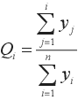and y_i is the value of variable y

(e.g. GDP per capita, unemployment rate, etc.) in region j when ranked from low (y₁) to high (y_N) among all regions within a country.

The index ranges between 0 (perfect equality: y is the same in all regions) and 1 (perfect inequality: y is nil in all regions except one).

Interpretation: The index assigns equal weight to each region regardless of its size; therefore differences in the values of the index among countries may be partially due to differences in the average size of regions in each country. Only countries with more than four regions are included in the computation of the Gini index.

Malmquist decomposition

Definition: The Malmquist index allows the decomposition of the productivity growth of a region between two effects, the frontier shift effect which is the change of regional productivity related to the gain of productivity of the frontier, and the catch-up effect which is the acceleration of the productivity of the region towards the frontier. The frontier in this publication is defined, by country, as the top 10% regions with the highest GDP per employee until the equivalent of 10% of national employment is reached. The frontier at OECD level is the simple average of each country’s frontier.

Productivity growth = frontier shift-effect × catch-up effect

The frontier-shift effect is the change of the frontier's productivity slope over the two periods (t) to (t+1), and the catch-up effect is defined by:

Where AC and DE are the theoretical levels of employment that region O should have, in order to have the same level of productivity as the frontier, in respect of the levels of its GDP in t and t+1. AO₁ and DO₂ are the levels of employment of the region O respectively in t and t+1. The productivity growth of the region.

Interpretation: If the region has reduced its productivity gap with the frontier (it has caught-up), the catch-up effect is above 1, and below 1 when the region has increased the productivity gap (it hasn’t caught-up) compared to the frontier's productivity.

Methodology to adjust GDP, total employed and unemployed at metropolitan level

The proposed methodology uses the socio-economic values (GDP, employment and unemployment) in TL3 regions as data inputs (see exceptions in Annex B) and the distribution of population based on census data.

In comparison to previous editions of Regions at a Glance, the methodology to adjust socio-economic data to metropolitan areas has evolved from the use of raster population data (i.e. Landscan) to municipal population census data as the input data source. This change has allowed the use of more up-to-date data (census data c.a. 2011) as well as the use of harmonised municipal boundaries over time. Indeed, long time-series have been generated using consistent boundaries of municipalities between the two census data points by using GIS techniques.

The suggested methodology is composed of three main steps:

• intersect the municipal boundaries with the TL3 boundaries by the use of GIS techniques;

• attribute each municipality a GDP value by weighting for the population in each municipality; and

• calculate the sum of municipalities’ GDP values belonging to each metro area.

An improved method would be to use employment data rather than population data in step 2. For example, the United Kingdom Office for National Statistics provides income estimates at ward level down-scaling the regional values through various variables including household size, employment status, proportion of the ward population claiming social benefits, and proportion of tax payers in each of the tax bands, etc. A similar method is used by the U.S. Bureau of Economic Analysis to estimate the GDP for U.S. Metropolitan Statistical Areas. The Federal Statistical Office of Switzerland used CLC-Data-Classes urban continuous fabric, urban discontinuous fabric and industrial or commercial units for all neighbouring countries by calibrating with other data to estimate data for jobs in grid cells. However these types of data input are not available in most OECD countries therefore a simpler solution was adopted.

A similar technique is applied to estimate employment and unemployment in metropolitan areas with working age population (15-65 years old) used as data input in step 2.

It has to be noted that the estimates of GDP, employment and unemployment in the metropolitan areas do not adhere to international standards; the comparability among countries relies on the use of the same methodology applied to areas defined with the same criteria.

Methodology to measure the annual exposure to air pollution in regions and metropolitan areas

The estimated average exposure to air pollution (PM_2.5) is based on GIS-based methodology at TL2 and metropolitan level using the satellite-based PM_2.5 estimates of van Donkelaar et al. (2014) at 0.1^o x 0.1^o geographic grid resolution. The method used to produce the estimates is the following:

• the satellite-based of air pollution at 1km² are multiplied by the population living in that area (using a 1km² resolution population grid);

• the exposure to air pollution in a region (or a metropolitan area) is given by the sum of the population weighted values of PM_2.5 in the 1km² grid cells falling within the boundaries of the region (metropolitan area); and

• finally, the average exposure to PM_2.5 concentration in a region is given by dividing this aggregated value by the total population in the region.

This indicator is derived from global satellite observations of PM concentration. It has the advantage of being computable globally without requiring country capacity investments in data collection.

Theil entropy index

Definition: Regional disparities are measured by a Theil entropy index, which is defined as:

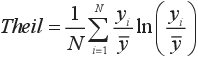
Where N is the number of regions in the OECD, y_i is the variable of interest in the i-^th region (i.e. household income, life expectancy, homicide rate, etc.) and  is the mean of the variable of interest across all regions.

The Theil index can be easily decomposed in two components: one is the disparities within subgroups of regions – where for example is subgroup is identified by a set of regions belonging to a country; another one is the disparities between subgroups of regions (i.e. between countries). The sum of these two components is equal to the Theil index.

In order to decompose the Theil index, let’s start by assuming m groups of regions (countries). The decomposition will assume the following form:

Where the first term of the formula is the within part of the decomposition it is equal to the weighted average of the Theil inequality indexes of each country. Weights, s_i, are computed as the ratio between the country average of the variable of interest and the OECD average of the same variable. The second term is the between component of the Theil index and it represents the share of regional disparities that depends on the disparities across countries.

Interpretation: The Theil index ranges between zero and ∞, with zero representing an equal distribution and higher values representing a higher level of inequality.

The index assigns equal weight to each region regardless of its size; therefore differences in the values of the index among countries may be partially due to differences in the average size of regions in each country.