Reader’s guide
The organising framework
Regions at a Glance 2016 addresses two questions:
-
How OECD regions perform in a wide range of well-being outcomes and what progress have regions made towards more inclusive and sustainable development, compared to the past and compared with other regions?
-
Which factors drive the performance of regions, and what local resources could be better mobilised to increase national prosperity and people’s well-being?
The first question is addressed in Chapter 1, which reveals the variety of regional performance, within and across countries. The framework for measuring well-being at the regional level considers a combination of individual characteristics and local conditions, to get closer to what people experience in their life. It has been conceived to improve policy coherence and effectiveness by looking at eleven dimensions, those that shape people’s material conditions (income, jobs and housing) and their quality of life (health, education, access to services, environment, safety, civic engagement and governance, community, and life satisfaction). These dimensions are gauged through indicators of “outcomes”, which capture improvements in people’s lives. For example, health is measured by the regional average life expectancy at birth, rather than public expenditure for health (input indicator) or number of doctors per population (output indicator). The well-being indicators chosen for 9 of the 11 dimensions are objective indicators that together provide a snapshot of the development of a region and, when possible, how the results are distributed among different population groups (elderly, young, women, foreign-born, etc.). For the first time in this publication two additional well-being dimensions are included, community and life satisfaction, and measured by self-reported indicators (or subjective indicators), where respondents are asked to evaluate their life or certain domains of their life.
Answering the second question can inform the design of effective strategies to improve the contribution of regions to aggregate performance and can suggest policy interventions to unlock complementarities among efficiency, equity and environmental sustainability objectives. Chapters 2, 3 and 4 – “Regions as drivers for national competitiveness”, “Subnational government finance and investment for regional development”, and “Inclusion and sustainability in regions” – showcase local resources, whether human capital, infrastructure, social capital, financial means, that can be mobilised to improve well-being outcomes.
Throughout the publication regional economies and societies are looked at through two lenses: the distribution of resources over space and the persistence of regional disparities over time. More precisely:
-
Distribution of resources over space is assessed by looking at the proportion of a certain national variable concentrated in a limited number of regions, corresponding to 20% of the national population and how much these regions contribute to the national change of that variable. For example, the OECD regions with the largest gross domestic product (GDP) and corresponding to 20% of the total population generated 26% of OECD GDP in 2013.
-
Regional disparities are measured by the difference between the maximum and the minimum regional values in a country (regional range), by the Gini index or by the Theil general entropy index,1 which give an indication of inequality among all regions. In Chile, Greece, Italy, Mexico, Portugal, Spain and Turkey, for example, the regional difference in the share of workforce with at least secondary education was higher than 20 percentage points in 2014.
Geographic areas utilised
Traditionally, regional policy analysis has used data collected for administrative regions, that is, the regional boundaries within a country as organised by governments. Such data can provide sound evidence on the contribution of regions to national performance as well as on the persistence of disparities within a country. They show, for example, that during the past 15 years more than 30% of growth in GDP, employment and population within the OECD is attributable to a small number of regions. At the same time, the places where people live, work and socialise may have little formal relationship to the administrative boundaries around them, for example: a person may inhabit one city or region but go to work in another and, on the weekends, practice a sport in a third. Regions interact through a broad set of linkages such as job mobility, production systems, or collaboration among firms. These often cross local and regional administrative boundaries. The analysis, therefore, should take into consideration, in addition to the administrative boundaries of a region, also its economic or social area of influence known as the functional region (Figure 1). The notion of functional region can better guide the way national and city governments plan infrastructure, transportation, housing, schools, and space for culture and recreation. In summary, functional regions can trigger a change in the way policies are planned and implemented, better integrating and adapting them to the local needs.
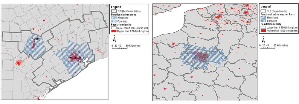
Note: These maps are for illustrative purposes and are without any prejudice to the status of or sovereignty over any territory covered by these maps.
Source: OECD calculations based on population density as disaggregated with Corine Land Cover, Joint Research Centre for the European Environmental Agency.
This publication features data both for administrative and functional regions according to international classifications, although the availability of data for the former is much more complete than for the latter.
Territorial level classification
Regions within the 34 OECD countries are classified on two territorial levels reflecting the administrative organisation of countries. The 391 OECD large (TL2) regions represent the first administrative tier of subnational government, for example, the Ontario Province in Canada. The 2 197 OECD small (TL3) regions are contained in a TL2 region. For example, the TL2 region of Aquitaine in France encompasses five TL3 regions: Dordogne, Gironde, Landes, Lot-et-Garonne and Pyrénées-Atlantiques. TL3 regions correspond to administrative regions, with the exception of Australia, Canada, Germany and the United States. All the regions are defined within national borders (See Annex A for the regional classification of each country).
This classification – which, for European countries, is largely consistent with the Eurostat NUTS 2010 classification – facilitates greater comparability of geographic units at the same territorial level.2 Indeed, these two levels, which are officially established and relatively stable in all member countries, are used as a framework for implementing regional policies in most countries.
Due to limited data availability, labour market indicators in Canada are presented for groups of TL3 regions. Since these groups are not part of the OECD official territorial grids, for the sake of simplicity they are labelled as non-official grids (NOGs) in this publication and compared with TL3 in the other countries. Germany has also a NOG category with the 96 Spatial Planning Regions, an intermediary level between the 16 Länders (TL2) and the 412 Kreise (TL3). The German NOG allows for a level of spatial disaggregation comparable to the other countries.
For the non-OECD countries, only TL2 regions have been identified for Brazil, China, Colombia, India, Peru, the Russian Federation and South Africa, whereas for Latvia and Lithuania, TL3 are derived from the European NUTS 3.
Definition of metropolitan areas
The OECD-EU definition of functional urban areas consists of highly densely populated urban centres and adjacent municipalities with high levels of commuting (travel-to-work flows) towards the densely populated municipalities. This definition overcomes previous limitations for international comparability linked to administrative boundaries. A minimum threshold for the population size of the functional urban areas is set at 50 000 population. The definition is applied to 30 OECD countries (with exception of Iceland, Israel, New Zealand and Turkey), and it identifies 1 197 urban areas of different sizes (see Figure A.5, Annex A for the detailed methodology).
The aim of this approach to functional urban areas is to create a methodology that can be applied across the whole OECD, thus increasing comparability across countries, unlike definitions and methodologies created within individual countries, which have been internally focused.3 In order to establish this cross-country methodology, common thresholds and similar geographical units across countries were defined. These units and thresholds may not correspond to the ones chosen in the national definitions. Therefore, the resulting functional urban areas may differ from the ones derived from national definitions and in addition the OECD functional urban delimitation may not capture all the local factors and dynamics in the same way as national definitions.
This publication includes data on metropolitan areas, which are defined as the functional urban areas with population above 500 000. According to this methodology, there are 281 metropolitan areas in the 29 OECD countries4 corresponding to 49% of total population in 2014.
Regional typology
Traditionally the OECD has classified TL3 regions as predominantly urban (PU), intermediate (IN), or predominantly rural (PR) regions. This typology is based on the percentage of regional population living in rural communities, combined with the existence of urban centres where at least one-quarter of the regional population reside. An extended regional typology has been adopted to distinguish between rural regions that are located close to larger urban centres and those that are not. The result is a four-fold classification of TL3 regions: predominantly urban (PU), intermediate regions (IN), predominantly rural regions close to a city (PRC) and predominantly rural remote regions (PRR). The distance from urban centres is measured by the driving time necessary for a certain share of the regional population to reach an urban centre with at least 50 000 people (see Annex A for a detailed description of the criteria and the resulting classification of TL3 regions). Due to a lack of information on the road network and service areas, the extended typology has not been applied to Australia, Chile and Korea. In 2014, the European Union modified the rural-urban typology, using 1 km population grids as building blocks to identify rural or urban communities, with the aim of improving international comparability; for the OECD-EU countries this rural-urban typology is presented in the publication.
While the rural-urban typology is calculated only for the lower territorial level (TL3) we are also interested in characterising TL2 regions according to the distribution of population in more rural or urban areas. For this purpose, we use the share of the regional population living in functional urban areas of different population sizes located in the region. This classification has the advantage of overcoming the urban-rural split and better capturing the contiguity of urban and rural life. In this publication, a TL2 region is classified as mostly urban if more than 70% of its population lives in a functional urban area located within the TL2 region. It should be noted that, due to lack of commuting data, functional urban areas are not identified in Iceland, Israel, New Zealand and Turkey. Therefore, the classification of mostly urban TL2 regions is not applied to these four countries.
Sources of data for territorial statistics
OECD Regions at a Glance 2016 includes a selection of indicators from the OECD Regional Database, the OECD Regional Well-Being Database, the OECD Metropolitan Areas Database and the OECD Subnational Government Finance Database.
Most of the indicators presented in Chapters 1, 2 and 4 (TL2 and TL3 regions) come from national official sources, following internationally common methods for cross-country comparability. At the same time, regional and local data are increasingly available from a variety of sources: surveys, geo-coded data, administrative records, big data, and data produced by users. While countries have started to make use of the various sources to produce and analyse data at different geographic levels, significant methodological constraints still exist, making it a challenge to produce sound, internationally comparable statistics linked to a location. These constraints include both the varying availability of public data across OECD countries and the different standards used by National Statistical Offices in defining certain variables. Such constraints are even larger in non-OECD countries, where the production and usability of geo-coded information could be one solution to improve statistical evidence for different policy uses, such as the monitoring of Sustainable Development Goals. The trade-off between sound methodological estimations and international comparability should be always considered, as the latter depends on the commonly available information.
The indicators for the metropolitan areas presented in Chapters 1, 2 and 4 are derived by integrating different sources of data, making use of GIS and adjusting existing regional data to non-administrative boundaries. Two types of methods to obtain estimates at the desired geographical level are applied, both requiring the use of GIS tools to disaggregate socio-economic data. The first method makes use of satellite datasets (global layers) at different resolutions, which are always smaller than the considered regions. The statistics for one region are obtained by superimposing the source data onto regional boundaries. In these cases, the regional value is either the sum or a weighted average of the values observed in the source data within the (approximated) area delimited by the regional boundaries. This method has been applied, for example, to estimate air pollution (population-weighted average of PM2.5 levels) in metropolitan areas, TL3 and TL2 regions to compensate for the lack of international standards for statistics of environmental conditions in regions.
The second method makes use of GIS tools to adjust or downscale data, available only for larger geographic areas, to regularly spaced “grids” by using additional data inputs that capture how the phenomenon of interest is distributed across space. With this method, GDP, employment and unemployment have been estimated in metropolitan areas, with exception of Australia and the United States that provided economic and social statistics for the metropolitan areas (see Annex C for details on the methods to estimate indicators for metropolitan areas).
GIS-based methodologies were used to estimate not only environmental, but also socio-economic indicators (GDP and labour market), because these methods are less dependent on the type of information available in the different countries and, therefore, they enable good comparability of results among metropolitan areas in different countries. This choice, however, has the disadvantages of lack of precision for some estimates and difficulty in obtaining comparable measures over time so as to monitor improvements induced by targeted policies and behavioural changes. Specific data products enabling comparison of data over time need to be produced, and, in addition, international standards for the production of indicators from remote sensing observation could be developed.
The data of Chapter 3 refer to subnational governments, as classified according to the General Government Data of the OECD National Accounts. Subnational governments are defined as the sum of states (relevant only for countries having a federal or quasi-federal system of government) and local (regional and local) governments.
Finally, for the first time, micro data from the Gallup World Poll were used to produce regional (TL2) estimates for three well-being indicators in Chapter 1: perception of government corruption, life satisfaction, and social support network. Survey responses over the period 2006-14 were pooled together to increase the regional sample size, and data were reweighted to better fit the age-gender cohorts in the real population.
Further resources
The interactive web-based tool www.oecdregionalwellbeing.org/ allows users to measure well-being in each region, compare it against other OECD regions and monitor progress over time. Each region is assessed in 11 areas central to the quality of life: income, jobs, health, access to services, environment, education, safety, civic engagement and governnance, housing, social support network, and life satisfaction.
The different topics are visualised through interactive graphs and maps with a short comment. Regional eXplorer and Metropolitan eXplorer allow users to select from among all the indicators included in the OECD Regional and Metropolitan Areas databases and display them in different linked dynamic views such as maps, time trends, histograms, pie charts and scatter plots. The website also provides access to the data underlying the indicators and to the OECD publications on regional and local statistics.
The cut-off date for data included in this publication was February 2016. Due to the time lag of subnational statistics, the last available year is generally 2014 for demographic, labour market and subnational finance data and 2013 for regional GDP, innovation statistics and social statistics.
The statistical data for Israel are supplied by and under the responsibility of the relevant Israeli authorities. The use of such data by the OECD is without prejudice to the status of the Golan Heights, East Jerusalem and Israeli settlements in the West Bank under the terms of international law.
Acronyms and abbreviations
OECD Country codes
Other major economy codes
Notes
← 1. With the α coefficient equal to 1.
← 2. For European countries, the Eurostat NUTS 2 and 3 classifications correspond to the OECD TL2 and 3, with the exception of Belgium, Germany and the United Kingdom where the NUTS 1 level corresponds to the OECD TL2.
← 3. Some OECD countries have adopted a definition for their own metropolitan areas or urban systems that looks beyond the administrative approach. For example, Australia (Australian Bureau of Statistics, 2012), Canada (Statistics Canada, 2002) and United States (U.S. Office of Management and Budget, 2000) use a functional approach similar to the one adopted here, to identify metropolitan areas. Several independent research institutions and National Statistical Offices have identified metropolitan regions in Italy, Spain, Mexico and United Kingdom based on the functional approach.
← 4. The functional urban area of Luxembourg has a population below 500 000 inhabitants.