Impact of the crisis on regional economic disparities
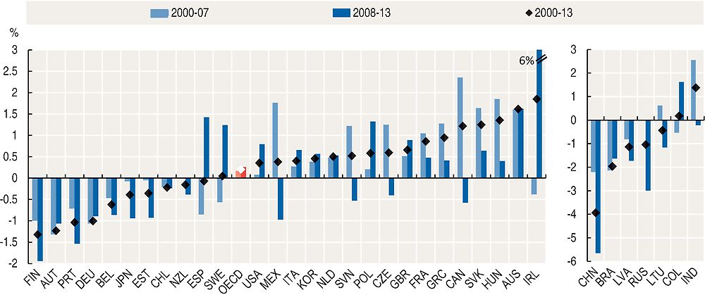
The evolution of the economic disparity within a country is here measured by the growth of the difference in gross domestic product (GDP) per capita between the richest 20% of regions and the poorest 20% of regions. This gap has grown in the OECD area at an average rate of 0.3% yearly in the period 2000-13 (Figure 2.42).
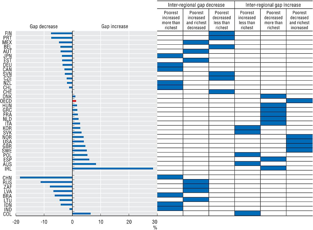
Regional economic disparities, however, can be very different between countries and for the periods before and after the economic crisis of 2008. Among the 27 OECD countries observed, 15 countries have grown in the inter-regional gap between richest and poorest regions for the period 2000-07, with Canada, Hungary, Mexico, the Slovak Republic and Australia having an increase of more than 1.5% per year. For the period 2008-13, this increase concerns 14 countries, with the biggest increases in inequalities located in Ireland and Australia. The crisis had a sharp effect especially in Ireland, Spain and Sweden, countries for which the inter-regional gap increased after the crisis where it was decreasing before, whereas for other countries like Mexico, Canada and Slovenia, the effect was the opposite (reduction after a growth) (Figure 2.43).
The interpretation of the evolution of the gap after 2008 depends on the evolution of the situation of poorest regions compared to richest. Japan, Germany, Canada, New Zealand and Chile had a reduction of the regional gap between 2008 and 2013 due to a better performance of the poorest regions, while in Finland, Portugal and Belgium, the reduction of the gap is due to a lower GDP per capita regression of poorest regions than richest (Figure 2.43).
The gap increased in Ireland, Spain and for six other countries due to higher recession of poorest regions compared to richest, whereas it increased in Australia, Poland, Slovak Republic and Korea due to faster growth in the richest regions (Figure 2.43).
GDP is the standard measure of the value of the production activity (goods and services) of resident producer units. Regional GDP is measured according to the definition of the System of National Accounts (SNA 2008). To make comparisons over time and across countries, it is expressed at constant prices (year 2010), using the OECD deflator and then it is converted into USD purchasing power parities (PPPs) to express each country’s GDP in a common currency.
GDP per capita is calculated by dividing the GDP of a country or a region by its population.
The top and bottom 20% regions are defined as those with the highest/lowest GDP per capita until the equivalent of 20% of the national population is reached.
Source
OECD (2015), OECD Regional Statistics (database), https://doi.org/10.1787/region-data-en.
OECD (2015), “Deflator and purchasing power parities”, OECD National Accounts (database), https://doi.org/10.1787/na-data-en.
Reference years and territorial level
2.42-2.43: GDP 2000-13; TL3.
Australia, Canada, Chile, Mexico and United States only TL2. Germany non-official grids.
Regional GDP is not available for Iceland, Israel and Turkey.
Figure notes
2.42: Denmark, Norway and Switzerland are excluded due to lack of data for 2000-13.
Information on data for Israel: https://doi.org/10.1787/888932315602.