Household income

In countries with rising disparities in household income, those disparities were mainly driven by faster income per capita growth in the most affluent regions.

Disposable income measures the capacity of households (or individuals) to consume goods and services. As such, it is a better indicator of material well-being of citizens than gross domestic product (GDP) per inhabitant. Regions specialised in natural resources production or regions that host the headquarters of large firms and that employ many workers living in other regions may display a very high GDP per capita, which does not necessarily translate into correspondingly high income of their inhabitants.

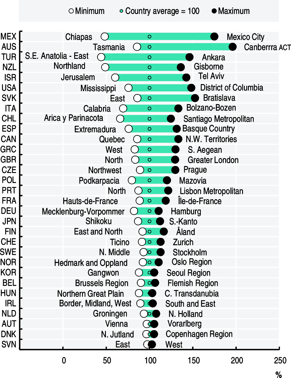
Disparities in regional disposable income per capita within countries are generally smaller than those in terms of GDP per capita. Even so, per capita disposable income in Mexico City (Federal District, Mexico), Canberra (Capital Territory, Australia), Ankara (Turkey), Gisborne Region (New Zealand) and Tel Aviv District (Israel), was in 2016 more than two times higher than in Chiapas, Tasmania, South-eastern Anatolia, East/ Northland Region and Jerusalem District, respectively. Similarly, in Australia, Mexico, Slovak Republic and the United States, inhabitants in the top income region had on average income that were over 50% higher than the national average (Figure 2.5).

2.5. Disposable income per capita in TL2 regions as a share of national average, 2016

 StatLink https://doi.org/10.1787/888933817067

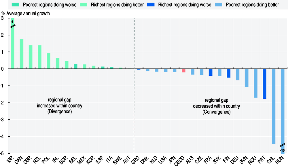
In roughly half of OECD countries, income disparities between the richest and poorest regions further increased during the last decade, this increase was particularly large in Israel, Canada and the United Kingdom where the ratio of income per capita between the top 10% and the bottom 10% of regions grew by more than 1.4% on average per year over the period 2011-16 (Figure 2.7). However, disparities decreased in various other countries, most notably in Hungary, Chile and Portugal. In countries with decreasing regional disparities, income convergence was predominantly driven by larger growth in the bottom regions. Analogously, regional divergence in income was generally driven by above average increases in disposable income in the richest regions, with some exception like Belgium, Spain and Italy (Figure 2.7).

2.6. Gini of disposable income within large regions (TL2), 2014

 StatLink https://doi.org/10.1787/888933817086

2.7. Evolution of the regional gap in disposable income per capita, 2011-16

Evolution of the ratio top 10% over bottom 10% large regions, and reason for the change

 StatLink https://doi.org/10.1787/888933817105

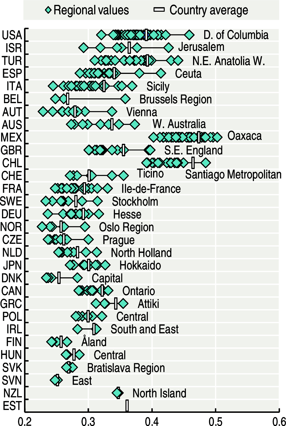
Differences in income are not only observed across regions, but also for households living in the same region. Levels of income inequality within regions differ, and these differences are particularly high in all large OECD countries as well as in some small countries with a dominant urban centre. For example, the difference between the Gini coefficients of the District of Columbia and the state of Utah in the United States (around 0.14) is of the same magnitude of the difference in the Gini coefficient between Mexico and the OECD average (Figure 2.6).