4. Good practices for developing standard mortality tables for retirement income arrangements

4.1.1. Understand historical patterns to inform future expectations

Understanding the trends in mortality and life expectancy is important to inform decisions regarding the selection and calibration of the models used to develop mortality assumptions. Economic and political contexts as well as societal trends can influence the historical trend of mortality, and changing contexts mean that certain historical experience may not always be an appropriate base for future expectations. Understanding the specific drivers of mortality in these contexts can help to inform whether observed trends will continue or whether changes are likely, providing a rationale for longer-term expectations regarding an acceleration or deceleration of improvements in life expectancy. In addition, an analysis of patterns for different groups of the population can aid in determining whether expectations might be different for the pensioner or annuitant population of interest.

Economic context can have a material influence on the speed of mortality improvement, particularly for countries that are rapidly developing. Current OECD countries who were lagging behind the OECD average life expectancy in the 1960s have since gained significant ground as they developed economically and their life expectancy caught up with the level observed in other OECD countries. Chile, Colombia, Costa Rica, and Korea, whose life expectancies at birth lagged at least 10 years behind the then-OECD average, have since caught up to the current OECD average life expectancy of just over 80 years, with Korea even exceeding this level (OECD, 2021[1]). Indeed, life expectancy is highly correlated with economic development, as Figure ‎4.1 clearly shows. Once the life expectancy of developing countries reaches that of economically advanced countries, the rapid growth will be likely to slow to the rate observed in the latter countries rather than continuing its rapid progression indefinitely into the future.

Figure 4.1. Life expectancy and GDP per capita, 2018

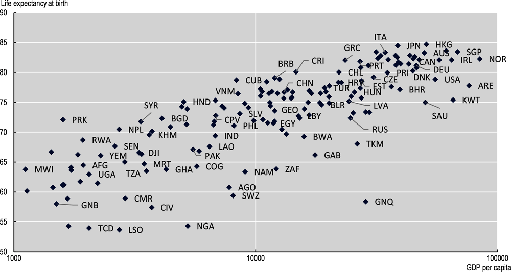
Note: GDP per capita is measured in 2011 international dollars, which corrects for inflation and cross-country price differences.

Source: Data from “Life Expectancy” Published Online at OurWorldInData.org: https://ourworldindata.org/life-expectancy

Political context can also influence the direction of trends in life expectancy. Shifts in political regimes, for example, can lead to clear breaks in historical patterns. The trends in life expectancy of Eastern European and Baltic countries illustrate the influence of the political context. Figure ‎4.2 shows that after years of stagnation, many of these countries experienced accelerated increases in life expectancy following the collapse of the Soviet Union, breaking with earlier observed trends.

Figure 4.2. Life expectancy at birth in selected Eastern European countries, 1950-2019

Source: Data from “Life Expectancy” Published Online at OurWorldInData.org: https://ourworldindata.org/life-expectancy

Breaks in historical mortality patterns may also be temporary. The COVID-19 pandemic led to significant excess mortality over 2020 and 2021. However, these spikes in mortality should largely be anomalous, with mortality levels returning to their pre-COVID-19 levels and trajectory. As such, it may be prudent to omit these years from any calibration of mortality going forward, as these high levels of mortality are not expected to continue for those who have survived the pandemic. Indeed, in response to the pandemic, the latest mortality projections model developed by the Continuous Mortality Investigation (CMI) in the United Kingdom allows users change the weight given to specific years in the calibration of the model (CMI, 2021[2]).

Specific policy initiatives can also affect life expectancies. For example, increased health care expenditure is strongly correlated with higher life expectancies, as seen in Figure ‎4.3. As such, policy initiatives that aim to increase public health care spending, such as the introduction of universal health care, should have a positive impact on life expectancy trends. Other policies aim to encourage more healthy behaviours, which can also have a direct impact on life expectancy. Cigarette taxes, for example, have been effective at reducing the prevalence of smoking, particularly for young adults and lower socio-economic groups (Sharbaugh et al., 2018[3]; Wilkinson et al., 2019[4]).

Figure 4.3. Life expectancy and health care expenditure, 2014

Note: Total health care expenditure per capita is adjusted for price differences between countries and for inflation and measured in international dollars.

Source: Data from “Life Expectancy” Published Online at OurWorldInData.org: https://ourworldindata.org/life-expectancy

An understanding of the specific drivers underlying the observed historical patterns can better inform future expectations and provide a rationale for why changes could be expected. In many countries, reduced improvements in mortality from cardiovascular diseases have been a large driver in the overall slowdown in improvements observed over the last decade in many high-income countries (OECD/The King's Fund, 2020[5]). Furthermore, while declining smoking rates were contributing to rapid mortality improvements, rising obesity as well as increased rates of diabetes are now offsetting some of these gains. Increased mortality from dementia at the oldest ages is also a concern, and is contributing to these negative trends. In Canada and the United States, deaths from drug overdoses have been a significant driver of the slowdown in mortality improvements (Ye et al., 2018[6]; Case and Deaton, 2017[7]). In Mexico, the stagnation of life expectancy since around 2000 has been mainly due to high rates of violence and homicide (Alvarez, Aburto and Canudas-Romo, 2019[8]). Identifying the direction of these types of drivers can provide an indication of whether long-term improvements could be higher or lower than historical trends imply.

The evolution of the distribution of lifespans can provide some insight as to where there is the most room for future improvement, the extent to which the maximum lifespan may be increasing, and the extent of longevity inequalities within the population. Where the left side of the distribution has decreased substantially, mortality improvements are more likely to shift to older ages where there is more room for additional improvements. A rightward shift of the distribution over time would indicate that the maximal age of survival is still increasing. A compression of the curve around the modal age of death would indicate a reduction in the variance of lifespans and therefore a likely reduction of longevity inequalities within the population. For example, Figure ‎4.4 shows a significant decrease in deaths below age 65 in Japan since 1960, accompanied by an increase in both the modal and maximal age of death.

Figure 4.4. Distribution of the age at death in Japan, 1960-2018

Source: Data from the Human Mortality Database: www.mortality.org.

Looking at the patterns of mortality improvements for different subgroups of the population will provide clearer insight as to any underlying inequalities in longevity and how longevity trends may differ across population subgroups. Some jurisdictions, such as Denmark, the United Kingdom and the United States, have seen the differences in life expectancy across socio-economic groups increasing over the last decades (Cairns, 2019[9]; Wen, Cairns and Kleinow, 2020[10]; Case and Deaton, 2017[7]). This is relevant to pensioner and annuitant populations, who tend to be from higher socio-economic groups, as they may experience more rapid mortality improvements than observed on average for the general population. Changes in certain mortality drivers could also imply a change in any underlying inequalities in the population. In many countries, the lower life expectancy of more disadvantaged populations is linked to unhealthy behaviours and habits such as smoking, lack of exercise, or drug use (Cairns, 2019[9]; Geronimus et al., 2019[11]; Tarkiainen et al., 2011[12]). It would therefore be likely that any improvement in these negative trends would be accompanied by a reduction in longevity inequalities across socio-economic groups.

4.1.2. Determine the granularity of assumptions given the availability of data and the purpose for which the assumptions will be used

Mortality experience can vary widely across different subgroups of the population. As such, mortality assumptions often differentiate between select groups. The level of granularity of assumptions will depend on the relevance of the indicator, the data available on which to calibrate the assumptions, as well as the purpose for which they will be used.

In all contexts, age and gender are the most relevant variables to consider when deciding the granularity of assumptions. At a minimum, mortality assumptions systematically account for differences in mortality across age, as mortality generally increases exponentially with age. Mortality also differs significantly between genders, with females normally having lower mortality than males at all ages within the same population group. At birth, women in OECD countries can expect on average to live around five-and-a-half years longer than males, but this difference can even exceed ten years (OECD, 2021[1]). Women aged 65 can expect to live over three years longer than their male counterparts in the OECD (OECD, 2022[13]). Given these differences, age and gender are the most common variables by which to differentiate mortality assumptions.

Variables indicating the socio-economic status of the individual may also be relevant, as higher socio-economic groups tend to have significantly higher life expectancy than those in lower socio-economic groups, even at older ages (OECD, 2016[14]). Furthermore, pensioner and annuitant populations tend to have a higher socio-economic level than the general population on average, with populations of voluntary annuitants typically demonstrating the largest differences from the population average. Common indicators used to differentiate among socio-economic groups for standard mortality tables are the level of pension income, the type of worker (e.g. blue or white collar), or geographical location.

Other indicators may aim to differentiate among types of beneficiaries. This could involve setting separate assumptions for members of public schemes and private schemes, or whether the pensioner is the original beneficiary or the surviving beneficiary. The extent to which mortality differs between these groups may depend on the particular context in which these schemes operate.

Mortality assumptions may also vary by some indicator of health. Distinct mortality assumptions are often used for smokers or for disabled populations, for example.

Developing separate assumptions for different groups requires sufficient data on which to base these assumptions. In many cases, there may not be sufficient data even if there is some evidence of substantial differences in mortality. For example, female disabled and male survivor beneficiaries tend to both be very small populations compared to the same groups of the opposite gender, largely driven by the historically male-dominated labour force covered by asset-backed pension arrangements. Where there is insufficient data, approximations may be used to adjust the mortality assumptions for other groups. For example, the CPM mortality tables in Canada provide factors to adjust the base mortality rates to the desired income band. In Peru, the mortality of the female disabled population is derived from the general population mortality based on the percentage of excess mortality that the male disabled population demonstrates.

The appropriate level of granularity also depends on the purpose for which the mortality assumptions will be used. Mortality assumptions used to determine retirement incomes are often unisex so as to not disadvantage women. In certain contexts, the use of socio-economic variables may also be considered discriminatory. On the other hand, income or health measures could be used as a way to increase the retirement income for more disadvantaged populations.

Mortality assumptions used for the purpose of calculating liabilities and reserves to secure future retirement incomes may be more granular so as to ensure a more accurate estimation of the level of assets needed to be set aside to finance future retirement incomes. As such, even if unisex mortality assumptions are used to calculate retirement incomes, the calculation of reserves usually relies upon separate assumptions for each gender. To capture the socio-economic gradient of mortality, assumptions used for reserving are also often based on pension amounts rather than individual lives.

The level of granularity of assumptions may also be different for the base assumptions and the mortality improvement assumptions. Mortality improvement assumptions usually only distinguish between ages and gender, whereas base mortality assumptions can vary by several additional variables.

4.1.3. Allow for flexibility to adapt assumptions where appropriate for their purpose

The level of standardisation required for mortality assumptions will depend in part on the purpose for which they are used. Standard mortality tables may serve as a basis for calculating retirement incomes or reserve requirements, or they may serve as a benchmark or reference from which to tailor assumptions to a specific population.

The use of standard mortality assumptions may be preferable where there is a need for consistency and comparability. This may be the case, for example, where standard assumptions are used to calculate the allowed level of programmed withdrawal, as in Chile, or where used for financial reporting or tax purposes, as in the United States.

Nevertheless, more accuracy may be preferred where the mortality assumptions are needed to value liabilities or for risk management purposes. Here, entities should be able to adapt the standard assumptions to better reflect the mortality of their actual pensioner or annuitant population if they can justify a different level of mortality based on experience. While many jurisdictions require standard tables as a minimum basis for valuation, this could potentially discourage providers from creating products to serve markets with lower life expectancies. Therefore, providers should ideally be able to adjust the standard assumptions in either direction so long as it is justifiable. Chile and Denmark take this approach, and providers are required to justify any deviation in assumptions from the benchmark mortality rates established by the supervisor.

4.1.4. Be open to innovative approaches

It may not always be possible or desirable to use traditional approaches to model mortality and develop standard mortality tables. The modelling of mortality is an evolving field, with new approaches being developed to overcome challenges relating to a lack of data or experience, or to better align assumptions with realistic expectations.

The lack of available or reliable data can be a major hurdle in the development of mortality tables, particularly for small pensioner or annuitant populations. Overcoming this limitation typically involves a significant amount of expert judgement. However, emerging techniques for data analysis, such as machine learning, are starting to be used to improve mortality estimates where data is lacking and to reduce the reliance on expert judgement alone.

Machine learning techniques are also starting to be applied to the calibration of existing mortality models to improve mortality estimates. These techniques can aid in the selection of data or the optimisation of parameters to improve the model’s fit and the accuracy of the modelled mortality rates, for example.

4.2.1. Calibrate assumptions for baseline mortality on data that is as similar as possible to the target population

Mortality differs widely across different populations groups, so it is important to calibrate baseline mortality assumptions on data that reflects the actual mortality of the target pensioner or annuitant population to whom the assumptions will apply. Ideally, assumptions will rely on data from the target population itself. However, these populations are sometimes too small to reliably calibrate assumptions, so larger populations for whom more data is available are often used. In this case, adjustments may be needed to ensure that the calibrated assumptions will reflect the expected mortality of the target population.

At a minimum, assumptions should rely upon mortality data from the same jurisdiction as the target population, as the differences in life expectancy across countries can be large. Among OECD countries, life expectancy at age 65 ranges from 17.9 years in Hungary to 24.6 year in Japan for women, and from 13.6 years in Lithuania to 20.2 years in Iceland for men (OECD, 2022[13]). This is a difference of over six years for both genders, which is very significant when assessing how long retirees can expect to live and how much they will need to finance their retirement.

Life expectancy also varies significantly across groups within a given jurisdiction, so the calibration of assumptions should rely upon a population within the jurisdiction that is representative of the target population, where possible. Pensioners and annuitants in particular tend to be better off than the general population on average, and as such tend to have life expectancies higher than the general population. In practice, baseline mortality assumptions for pensioner or annuitant populations tend to result in life expectancies at age 65 of around 2 to 2.5 years higher on average than the general population.1 Where these populations are smaller relative to the general population, as tends to be the case for annuitant populations, these differences can be even larger.

One approach to account for these differences is to rely upon a proxy population that demonstrates the same characteristics as the target population to calibrate baseline mortality assumptions. This approach can be useful when the target population is a specific subset of a population for which data is available. In Lithuania, for example, the public annuity provider created in 2020 uses mortality assumptions based on mortality data for higher-earning pensioners covered by the public system to proxy the expected mortality of new annuitants.

However, accurately defining a proxy population may be difficult given the data available, so lacking data for the target population, the general population most often serves as the basis for the calibration of baseline mortality assumptions. Where the general population is not representative of the target population, adjustment factors – or selection factors – are also needed to account for the lower expected mortality of the pensioner or annuitant population. These factors are normally based on the observed magnitude of differences in mortality between the pensioner or annuitant population and the general population in other jurisdictions where data is more readily available.

Calibrating selection factors on experience in other jurisdictions nevertheless requires some caution, as the level of coverage of any given type of scheme in a specific jurisdiction can substantially affect the size of the selection factor. Figure ‎4.5 demonstrates the negative relationship between coverage and the magnitude of the difference in life expectancy at age 65 between the general population and the pensioner/annuitant population. In view of this, it would not be advisable for a jurisdiction having a small population of annuitants, for example, to base selection factors solely on the UK pensioner population, where closer to half the population is covered.

Figure 4.5. Relationship between coverage and extent of mortality selection at age 65

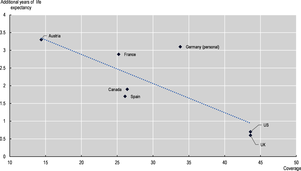
Note: The population that the data on coverage represents does not exactly correspond to the population to which the mortality tables apply. The countries shown are selected based on the likelihood that these two populations more closely correspond to each other.

Source: Coverage figures from (OECD, 2019[15]). Selection factors are own calculations.

The magnitude of selection observed typically also varies across ages and between genders. Differences generally increase until around age 60 and decrease thereafter. Differences tend to be larger for men than for women.

4.2.2. Graduate baseline mortality considering available data and the desired fit and smoothness

Standard mortality tables should provide smooth estimates of mortality rates across ages. This requires graduating the raw baseline mortality rates calculated directly from the data. The selection of the graduation model should consider the characteristics of raw mortality rates as well as the trade-off between fit and parsimony.

The age range over which the baseline mortality rates are calibrated may inform the choice of graduation model. The Gompertz model is a simple model that captures the typically observed pattern of an exponential increase in mortality with age. However, this pattern is most appropriate for ages above around 65. If the graduation needs to extend to younger ages, variations on the Gompertz model that account for differing patterns at young and middle ages may be more appropriate for smoothing mortality across all ages. The Gompertz-Makeham model better reflects excess mortality at middle ages, while the Heligman-Pollard better captures mortality patterns for younger ages.

Alternative models, such as the Whittaker-Henderson model, can fit the pattern of the raw data more closely and across years as well as ages, but at the expense of parsimony. The Whittaker-Henderson model is commonly used to smooth baseline mortality assumptions for standard tables, but involves fitting significantly more parameters compared to simpler models. It also requires more judgment to set the user-defined parameters, such as those regulating the smoothness of the graduated mortality rates. Statistical tests, in particular information criteria, can aid in the selection of the appropriate model to balance the trade-off between fit and parsimony.

Where the same population is the basis to calibrate both baseline mortality assumptions and future mortality improvements, it is possible to use a fully integrated model that fits past mortality and simultaneously projects it into the future. In selecting these types of models, the trade-off between fit and parsimony remains applicable.

4.2.3. Consider the expected pattern of mortality when extrapolating assumptions to the oldest ages

It is necessary to extrapolate the graduated rates for old ages to derive the mortality assumptions for the oldest ages – e.g. beyond age 90 or 95 – as the data at these ages are normally insufficient to calibrate mortality rates. The model chosen to do this should result in a plausible pattern of mortality at the oldest ages, in line with any trends observed at the national or regional level.

There are conflicting views regarding the pattern of mortality at the oldest ages, particularly ages over 110 where there is insufficient data on which to base any robust analysis. One side argues that mortality rates continue increasing exponentially with age, while the other side argues that mortality rates eventually plateau at around age 110 (Gavrilov, Gavrilova and Krut’ko, 2017[16]; Gampe, 2010[17]). In practice, both views are taken in the development of standard mortality tables. Those taking the former view most commonly use some variation of the Gompertz model to extrapolate mortality to the oldest ages. For the latter view, a logistic model such as the Kannisto model is often used.

The selected model should result in a pattern of mortality at the oldest ages that is consistent with expectations and available evidence. The extrapolated mortality rate should not reach 1 at an age below the desired maximum age (see the following guideline). If assuming that mortality rates ultimately plateau, most available evidence suggests that the force of mortality plateaus between around 0.7 and 1.2, which translates into an annual probability of dying of around 50% to 70%.

Input parameters to calibrate the model can also influence the pattern of the extrapolated rates to shape them in the desired direction. These parameters can include the age range over which the model is calibrated, the constraints imposed such as the maximum age, or any external (e.g. population) mortality table referenced.

4.2.4. Set the maximum age of the mortality table to ensure that assumptions will apply to all members of the target population

The mortality table should cover all of the ages that the target population includes, in particular the oldest of the population. If the target population includes individuals aged 115, the mortality table should include mortality assumptions at least to this age.

In practice, mortality tables normally assume an ultimate age beyond which there will be no survivors for the sake of practicality, regardless of the view taken on the pattern of mortality at the oldest ages. This ensures the ultimate run-off of any pension or annuity liabilities.

The ultimate age assumed, however, should be inclusive of everyone included in the target population to which assumptions apply. This is not always the case. Several standard mortality tables in OECD jurisdictions assume an ultimate age of 110 or lower, whereas individuals over this age may exist. Assumptions are still needed to apply to these oldest individuals regardless of how the mortality tables are used, whether to value liabilities or to calculate a retirement income.

Most standard mortality tables in OECD jurisdictions assume a maximum age of at least 120. Globally, no individual over the age of 120 is currently alive, and only one person has been verified as ever reaching an age older than 120.2

Nevertheless, this does not necessarily mean that the ultimate age of survival cannot be higher. Patterns in the evolution of distribution of lifespans of a population can inform assumptions regarding the maximum age of the mortality table. If this distribution has been shifting rightward, it could indicate that the maximum age of survival may still be increasing, thereby justifying a higher ultimate age than the oldest observed survivor.

4.3.1. Account for future mortality improvements in a way that reflects reasonable expectations

Standard mortality tables need to account for future expected improvements in mortality, as they add materially to the life expectancy of pensioners and annuitants. The way that mortality tables incorporate improvement assumptions should accurately reflect reasonable expectations regarding the impact that improvements will have on life expectancy.

The impact of mortality improvements on the calculation of life expectancy is significant. Mortality improvements represent on average around 1.5 additional years of life expectancy at age 65 relative to the life expectancy calculated using only current baseline mortality rates.3

The most realistic format with which to account for mortality improvements is a two-dimensional improvement scale that varies by both age and time. Indeed, this is the most common format for improvement assumptions included with standard mortality tables in the OECD. The way in which mortality tables take mortality improvements into account should accurately reflect their expected impact on life expectancy. In reality, mortality improvements are different across ages and emerge gradually over time. Each year, the mortality rate at a given age usually declines compared to the previous year. Furthermore, trends by age may not be constant over time, but may accelerate or decelerate.

Simplifications of two-dimensional improvements may be preferred in light of constraints to incorporate two-dimensional mortality assumptions into modelling, but this should not be a prevailing constraint given current technological capabilities. An alternative to a two-dimensional improvement scale is a one-dimensional scale that provides improvements by age but does not vary over time. Depending on the model used to calibrate the assumptions (e.g. extrapolative models such as the Lee-Carter model), this may not make a material difference in calculations compared to a two-dimensional improvement scale. However, age-shift methods that proxy the increased life expectancy of younger cohorts by simply assuming that they have a younger age are not very accurate (e.g. assuming that a 65-year-old in five years will have the same life expectancy as a 63-year-old today), and can become less accurate over time.

4.3.2. Choose a projection model compatible with future expectations taking into account the trade-off between transparency and complexity

A variety of models are available to calibrate mortality improvement assumptions, each of which demonstrates a range of advantages and drawbacks. Selection of the appropriate model will need to consider expectations regarding how mortality will evolve in the future and how to best match those expectations while minimising the level of complexity in the model. While complex models may better fit the data and result in mortality improvement assumptions that better align with realistic expectations, they can reduce the transparency of the model, thereby making it more difficult for the end-user to understand how assumptions were derived.

Mortality projection models that are commonly used to derive future improvement assumptions vary in how they reflect future expectations and are able to incorporate expert judgement. The simplest approach is to apply a linear regression to historical mortality rates to derive the historical trend, and extrapolate this trend going forward. Interpolative models incorporate more judgement regarding expected future trends, and assume improvements will eventually converge to an expected long-term rate of mortality improvement. Age Period Cohort (APC) models deconstruct the patterns of historical mortality along age, period and/or cohort dimensions to extrapolate future mortality rates. Multi-population models extend these approaches to simultaneously project mortality for two or more related groups.

A key question in selecting a model for projecting mortality forward is whether future mortality improvements will reflect past experience indefinitely, or whether mortality improvements are more likely to converge to some other rate in the long term. If taking the former view, modelling options include simple regression models or age-period-cohort (APC) models. Both of these approaches can also be incorporated into an interpolative model to accommodate the latter view of a convergence to a long-term rate of improvement. A multi-population model, which is often an extension of an APC model, is another option that can also assume convergence to a long-term rate based on some reference population.

Increased model complexity can allow the model to better account for the relationship of mortality rates across ages. Simple regression models extrapolate future mortality improvements based on linear regressions of log mortality rates by age (group). APC models, such as the Lee-Carter and Cairns-Blake-Dowd models, are extrapolative models that deconstruct mortality patterns along age, period, and potentially cohort dimensions. While APC models are more complex to fit and to explain than simple regression models, they are better able to capture the age structure of mortality improvements and maintain coherent mortality rates in future years. The inclusion of a cohort effect is not always justified however, and unless historical experience suggests that mortality patterns have been very different for specific cohorts, they may add unnecessary complexity to the model.

The level of complexity involved in interpolative models can vary widely, and is driven by the sub-models used for the graduation and interpolation of mortality rates. Interpolative models generally involve two main steps:

1. 1. Smooth historical mortality experience by fitting it to a model in order to establish an initial rate of mortality improvement by age.

2. 2. Interpolate the initial rates of mortality improvement to a long-term rate of improvement.

Interpolative models can employ several types of the models already discussed to smooth historical mortality experience. Both simple regressions and APC-type models can be fit to historical mortality rates to derive smoothed historical improvement rates. In addition, models such as the Whittaker-Henderson model, which is also common to establish baseline mortality rates, can be fit across two-dimensional historical mortality experience. The latter model is the most complex and involves more user input to fit, but is also able to better reflect the specific patterns in mortality observed. APC models involve less subjectivity than models like Whittaker-Henderson, but are still able to reflect the age structure of mortality rates, which is not possible with a simple regression model.

The interpolation of the initial mortality improvement to a long-term rate of improvement can also involve more or less complexity. The simplest approach is to apply a linear interpolation by age, but this ignores any differences in the speed of convergence across time or ages. More complex approaches allow for different convergence rates across period and cohort dimensions, or changes in the slope of convergence over time. However, this also involves significantly more judgement in setting the parameters for convergence.

Multi-population models are the most complex option for projecting future mortality improvements. They nevertheless offer a potential solution to model mortality improvements for smaller populations for whom there is not sufficient data to calibrate a model, or to ensure coherent mortality projections across several related populations (e.g. for males and females). However, they can more be difficult to calibrate and to understand.

Another consideration for assessing the desired model complexity is the extent to which stochastic longevity scenarios are needed for longevity risk assessments that are consistent with the mortality tables developed. If this is the case, APC models and their extensions (e.g. multi-population models) lend themselves more easily to stochastic projections.

Generally, the modelling of mortality improvements for the oldest ages can adopt a simpler approach. As with establishing baseline assumptions, there is not sufficient data at the oldest ages on which to calibrate robust assumptions for improvements. There is mixed evidence as to whether older ages have recently experienced positive mortality improvements, but there does seem to be consistent evidence that mortality improvements decrease with age. A common approach for standard mortality tables is therefore to simply assume that mortality improvements decrease to 0% at a certain age. Alternatively, the rates fitted to the projection model can be extrapolated in each future year to cover the oldest age groups.

4.3.3. Calibrate mortality projection models on a stable population representative of the target population

Mortality projection models should be calibrated on data from a population that is representative of the target population, and which has not been subject to any major shocks or shifts over the historical period selected for calibration.

As with baseline mortality assumptions, mortality improvement assumptions should be based on a population that is related to the target population of interest. There is not normally sufficient historical data for pensioner or annuitant populations on which to calibrate robust trends. General population mortality is commonly used to establish mortality improvement assumptions for standard mortality tables, with the assumption that the mortality of the pensioner or annuitant population should improve at the same rate as the population on average. Where evidence indicates that life expectancies across socio-economic groups are diverging, mortality improvement assumptions may include an additional selection factor to account for the higher expected improvements of pensioner and annuitant populations.

The impact of different policies on historical demographic patterns also need to be considered. Some policies affecting a population’s demographic composition can make it difficult to measure historical patterns on which to base future expectations. Israel’s relatively open immigration policy, for example, has led to high levels of immigration that reduces the stability in the demographic characteristics of the population, which could potentially distort any measurement of historical patterns of mortality improvement (Israeli Association of Actuaries, 2018[18]). Another example is in Chile, where a reform of the pension system in 2008 greatly expanded its coverage to lower income individuals, changing the socio-economic composition of the pensioner population (Pensiones, 2015[19]).

The historical period selected to calibrate the models used to derive improvement assumptions should not demonstrate any major breaks in trend and overall should reflect at least near-term expectations regarding future mortality improvement. Model calibration should therefore ideally refer to a period over which the average trend is relatively stable. It should also consider excluding large, anomalous shocks such as the years demonstrating excess mortality due to COVID-19.

Model calibration should also take into account the sensitivity of the model outputs to the selection of the historical period. Purely extrapolative models are generally more sensitive to the length of the historical period than interpolative models where initial improvement rates are reflective of the most recent fitted historical data.

4.4.1. Ensure coherency across different ages and groups

Mortality rates for different groups of the population consistently demonstrate certain relationships that the standard mortality table should reflect. As such, it is prudent to make sure that model outputs are coherent across different ages and population groups.

Mortality rates should generally increase monotonically with age. As a starting point, the model selected to graduate the baseline mortality assumptions should ensure that this is the case. A model that over fits the data, for example a Whittaker-Henderson model that does not put sufficient weight on smoothness, may result in a ‘bumpy’ mortality curve that does not demonstrate the expected pattern of increasing mortality with age. Mortality projections should also be coherent across ages. Projection models that do not impose a certain age structure may eventually distort the shape of the mortality curve across ages.

Male mortality should generally be higher than female mortality within the same population group. If this pattern is not apparent in the calibration of baseline assumptions, there is likely not sufficient data on which to develop robust assumptions. Any selection factors applied could also potentially distort the relationship of mortality across genders. Selection factors tend to be larger for males, so there could be a risk that their application could result in lower mortality for males than for females. The relationship between genders could also change over time as a result of higher projected mortality improvements for males. This is a particular risk when using extrapolative projection models, as the difference in life expectancy between men and women in many countries has been decreasing over the last few decades, meaning that males will have experienced higher mortality improvements than females.

The mortality for disabled populations should generally be higher than for healthy populations. This is because their underlying deteriorated health condition often leaves them more vulnerable to death, though this depends to a certain extent on the type of disability. A simple way to ensure that this relationship is not distorted in the future is to assume the same mortality improvement assumptions for both the healthy and disabled populations. This is a reasonable assumption, as the disabled population should benefit at least as much from the medical advances and external factors that are driving continued improvements in mortality for the healthy population.

While not an absolute constraint, evidence points to a convergence in mortality across population groups with age, whether between genders, across socio-economic groups, or for different categories of health. This is a result of a selection effect, whereby only the strongest and healthiest of the population survive to the oldest ages. This means that the differences in mortality across population groups should gradually diminish with age. The easiest way to ensure that this is the case is to reference a common mortality table when extrapolating mortality rates for different groups to the oldest ages.

4.4.2. Be transparent regarding modelling decisions

The modelling of mortality and development of standard mortality tables involves a considerable amount of judgement at each step of the process. The documentation for the development of the tables should identify areas where judgement was required and provide a rationale and justification for the modelling decisions made. It should also include information, such as sensitivity tests, to help the user understand the impact that the different decisions have had on the final assumptions. Ensuring transparency will help the user to determine whether the tables are appropriate for their intended use.

References

[3] Akinyemiju, T. (ed.) (2018), “Impact of cigarette taxes on smoking prevalence from 2001-2015: A report using the Behavioral and Risk Factor Surveillance Survey (BRFSS)”, PLOS ONE, Vol. 13/9, p. e0204416, https://doi.org/10.1371/journal.pone.0204416.
[8] Alvarez, J., J. Aburto and V. Canudas-Romo (2019), “Latin American convergence and divergence towards the mortality profiles of developed countries”, Population Studies, Vol. 74/1, pp. 75-92, https://doi.org/10.1080/00324728.2019.1614651.
[9] Cairns, A. (2019), Mortality Data By Socio-Economic Group, Region and Cause of Death: What Do the Patterns Tell Us?.
[20] Cairns, A. et al. (2019), “Modelling Socio-Economic Differences in the Mortality of Danish Males Using a New Affluence Index”, ASTIN Bulletin, Vol. 49/03, pp. 555-590, https://doi.org/10.1017/asb.2019.14.
[7] Case, A. and A. Deaton (2017), “Mortality and Morbidity in the 21st Century”, Brookings Papers on Economic Activity, Vol. 2017/1, pp. 397-476, https://doi.org/10.1353/eca.2017.0005.
[2] CMI (2021), CMI_2020 v01 methods.
[17] Gampe, J. (2010), “Human mortality beyond age 110”, in Demographic Research Monographs, Supercentenarians, Springer Berlin Heidelberg, Berlin, Heidelberg, https://doi.org/10.1007/978-3-642-11520-2_13.
[16] Gavrilov, L., N. Gavrilova and V. Krut’ko (2017), Mortality Trajectories at Exceptionally High Ages: A Study of Supercentenarians, Society of Actuaries.
[11] Geronimus, A. et al. (2019), “Weathering, Drugs, and Whack-a-Mole: Fundamental and Proximate Causes of Widening Educational Inequity in U.S. Life Expectancy by Sex and Race, 1990–2015”, Journal of Health and Social Behavior, Vol. 60/2, pp. 222-239, https://doi.org/10.1177/0022146519849932.
[18] Israeli Association of Actuaries (2018), Report of the Mortality Research Committee of the Israel Association of Actuaries on Mortality Improvements in Israel.
[13] OECD (n.d.), Life expectancy at 65 (indicator), https://doi.org/10.1787/0e9a3f00-en.
[1] OECD (n.d.), Life expectancy at birth (indicator), https://doi.org/10.1787/27e0fc9d-en.
[15] OECD (2019), “Coverage of funded and private pension plans”, in Pensions at a Glance 2019: OECD and G20 Indicators, OECD Publishing, Paris, https://doi.org/10.1787/983bdeef-en.
[14] OECD (2016), “Fragmentation of retirement markets due to differences in life expectancy”, in OECD Business and Finance Outlook 2016, OECD Publishing, Paris, https://doi.org/10.1787/9789264257573-11-en.
[5] OECD/The King’s Fund (2020), Is Cardiovascular Disease Slowing Improvements in Life Expectancy?: OECD and The King’s Fund Workshop Proceedings, OECD Publishing, Paris, https://doi.org/10.1787/47a04a11-en.
[19] Pensiones, C. (2015), Anexo N° 8 Nota técnica construcción tablas CB-H-2014 (hombres), MI-H-2014 (hombres), RV-M-2014 (mujeres), B-M-2014 (mujeres) y MI-M-2014 (mujeres), https://www.spensiones.cl/portal/compendio/596/w3-propertyvalue-9531.html.
[12] Tarkiainen, L. et al. (2011), “Trends in life expectancy by income from 1988 to 2007: decomposition by age and cause of death”, Journal of Epidemiology and Community Health, Vol. 66/7, pp. 573-578, https://doi.org/10.1136/jech.2010.123182.
[10] Wen, J., A. Cairns and T. Kleinow (2020), “Fitting multi-population mortality models to socio-economic groups”, Annals of Actuarial Science, pp. 1-29, https://doi.org/10.1017/s1748499520000184.
[4] Wilkinson, A. et al. (2019), “Smoking prevalence following tobacco tax increases in Australia between 2001 and 2017: an interrupted time-series analysis”, The Lancet Public Health, Vol. 4/12, pp. e618-e627, https://doi.org/10.1016/s2468-2667(19)30203-8.
[6] Ye, X. et al. (2018), “At-a-glance - Impact of drug overdose-related deaths on life expectancy at birth in British Columbia”, Health Promotion and Chronic Disease Prevention in Canada, Vol. 38/6, pp. 248-251, https://doi.org/10.24095/hpcdp.38.6.05.