
3. Tax revenue effects of Pillar Two
174. This chapter presents the analytical framework and data sources used by the OECD Secretariat to assess the effect on corporate tax revenues of Pillar Two. It also contains high-level estimates of the impact of Pillar Two at the global level and at the level of broad groups of jurisdictions. Pillar Two addresses remaining BEPS challenges and is designed to ensure that large internationally operating businesses pay a minimum level of tax regardless of where they are headquartered or the jurisdictions they operate in (OECD, 2020[1]).
175. The analytical framework presented in this chapter explores the implications of (i) several illustrative design and parameter options under Pillar Two, (ii) the interaction between Pillar One and Pillar Two and how this interaction can affect the revenue effects of Pillar Two, and (iii) potential behavioural reactions by multinational enterprises (MNEs) and governments to the introduction of Pillar Two. A number of design elements and parameters of Pillar One and Pillar Two will be the subject of future decisions by the Inclusive Framework. The Pillar One and Pillar Two design and parameter options considered in this chapter are only illustrative examples and should not be seen as prejudging any final decisions to be taken by the Inclusive Framework.
176. Similar to the framework used to assess the effect of Pillar One (see Chapter 2), the framework presented in this chapter spans more than 200 jurisdictions and combines a variety of micro- and macro-level data sources into a consistent structure. One central element of this structure is the set of data matrices described in detail in Chapter 5.
177. The framework is building on the best data sources available to the OECD Secretariat, and the underlying data has been subject to extensive checks and comparisons across data sources. The resulting estimates are nevertheless subject to a number of important caveats:
The assessment of Pillar Two revenue effects in this chapter is based on a number of simplifying assumptions on the design and implementation of Pillar Two, reflecting the challenges involved in modelling certain potential provisions of Pillar Two with the available data. In particular, the switch-over rule and the subject to tax rule have not been modelled, while the income inclusion rule and the undertaxed payments rule have been modelled only in a relatively stylised way. The potential effect of temporary or permanent differences between financial accounting profit and the Pillar Two tax base, and the effect of a loss carry-forward mechanism under Pillar Two (or any other profit smoothing mechanism) have not been taken into account. The modelling of a potential formulaic substance-based carve-out is based on a number of simplifying assumptions, as discussed further in this chapter.
The approach to estimating the effect of Pillar Two focuses on low-taxed profits in generally low-tax jurisdictions,1 but leaves aside potential “pockets” of low-taxed profit in generally higher-tax jurisdictions, due to limitations in the available data. The upper bound of the uncertainty ranges surrounding the estimates in this chapter has been increased to account for this uncertainty, as described further in this chapter.
Due to data limitations, the effect of certain provisions that may already allow jurisdictions to levy taxes on profit that would otherwise be subject to low levels of effective taxation (e.g. withholding taxes, CFC rules) is not taken into account in the modelling in this chapter, which could lead to overestimating potential revenue gains.
The data underlying the analysis have limitations in terms of coverage, consistency and timeliness. In particular, the reliance on aggregate data in certain parts of the analysis and for certain jurisdictions implies that some firm-level heterogeneities are overlooked, which could affect the results. Data on MNEs’ profit relates primarily to years 2016 and 2017. It therefore pre-dates some significant recent developments, including the implementation of various measures under the OECD/G20 Base Erosion and Profit Shifting project,2 the US Tax Cuts and Jobs Act (TCJA) and, more recently, the impact of the COVID-19 crisis. More specifically:
The implementation of the BEPS Action Plan is expected to reduce the amount of global low-taxed profit by reducing opportunities for MNEs to shift profit to low-tax jurisdictions. This reduces the potential revenue gains from Pillar Two.
Regarding the US TCJA, while no decision has been taken by the Inclusive Framework yet, the analysis assumes illustratively that the US Global Intangible Low Tax Income (GILTI) regime that has been in place since 2018 and results in a form of minimum tax on the foreign profit of US MNEs would “co-exist” with Pillar Two. Potential gains from Pillar Two presented in this chapter exclude US MNEs on the basis of the assumption that they would remain subject to GILTI and not be subject to the Pillar Two rules. Revenue gains from GILTI are discussed in section 3.8 of this chapter, based on ex ante estimates by the US Joint Committee on Taxation (US Joint Committee on Taxation, 2017[2]).
The COVID-19 crisis is likely to reduce the profitability of many MNEs – and, in turn, the amount of profit subject to Pillar Two – in the short and medium run, due to lower consumer demand, as well as potential difficulties with production (e.g. locked-down workers, supply chain disruptions, restrictions on travel). The longer term effect of the crisis on MNE profitability remains highly uncertain and will depend on the shape and speed of the economic recovery, as well as potential structural changes to the economy that the crisis may bring or accelerate (e.g. changes in the sectoral structure of economies, including faster-than-expected digitalisation of certain activities, as well as potential changes in the structure of global value chains and competition dynamics among firms).
The methodology takes into account, in a stylised way, potential strategic reactions by MNEs and governments to the introduction of Pillar Two. More specifically, the analysis focuses on (i) potential changes in MNEs’ profit shifting intensity, and (ii) potential tax rate increases in jurisdictions with an average effective tax rate (ETR) below the Pillar Two minimum rate. However, the exact nature and intensity of these reactions is difficult to anticipate with certainty, especially in the context of a coordinated multilateral tax reform, while existing studies are mainly based on jurisdiction-specific reforms. In particular, the exact location of MNE profits in a post-Pillar Two world is difficult to anticipate because MNE profit shifting schemes are often complex and could be modified in ways that are complex and difficult to anticipate following the introduction of Pillar Two.
The analysis in this chapter does not try to model other potential reactions by MNEs and governments, including potential changes in MNEs’ real investment decisions and policy reactions by other jurisdictions. The implications of Pillar One and Pillar Two on MNEs’ real investment decisions and on tax competition between jurisdictions are discussed in detail in Chapter 4. Overall, the assessment in Chapter 4 is that Pillar One and Pillar Two would have a small negative direct effect on global MNE investment that could be partly or even fully offset by positive indirect effects. In addition, a consensus-based multilateral solution involving Pillar One and Pillar Two would lead to a more favourable environment for investment and growth than would likely be the case in absence of an agreement by the Inclusive Framework (see Chapter 4). Still, Pillar Two could lead to significant increases in investment costs in jurisdictions where the ETR is currently below the potential level of the minimum rate under Pillar Two. This could significantly affect MNE investment in these jurisdictions and, in turn, affect CIT revenues, as well as revenues from other tax bases (e.g. personal income tax, value added tax) in these jurisdictions.
178. Given these caveats, the estimates based on the framework presented in this chapter should be interpreted as illustrating the broad order of magnitude of the impacts of Pillar Two, rather than precise point estimates. Actual gains from Pillar Two may differ from these ex ante estimates as these gains will ultimately depend on the final design and parameter decisions to be taken by the Inclusive Framework, the actual responses of MNEs and governments to the introduction of Pillar Two and the economic situation at the time of implementation. In light of this, the estimates presented in this chapter are expressed as ranges to reflect the uncertainty surrounding them. For simplicity, some intermediate results in this chapter are presented as point estimates, but the overall results in the final section are presented as ranges.
179. As described in the Pillar Two Blueprint report (OECD, 2020[1]), Pillar Two comprises a number of interlocking rules that seek to (i) ensure minimum taxation while avoiding double taxation or taxation where there is no economic profit, (ii) cope with different tax system designs by jurisdictions as well as different operating models by businesses, (iii) ensure transparency and a level playing field, and (iv) minimise administrative and compliance costs.
The principal mechanism to achieve this outcome is the income inclusion rule (IIR) together with the undertaxed payments rule (UTPR) acting as a backstop (the “GloBE rules”). The operation of the IIR is, in some respects, based on traditional controlled foreign company (CFC) rule principles and triggers an inclusion at the level of the shareholder where the income of a controlled foreign entity is taxed at below the effective minimum tax rate. It is complemented by a switch-over rule (SOR) that removes treaty obstacles from its application to certain branch structures and applies where an income tax treaty otherwise obligates a contracting state to use the exemption method. The UTPR is a secondary rule and only applies where a Constituent Entity is not already subject to an IIR. The UTPR is nevertheless a key part of the rule set as it serves as back-stop to the IIR, ensures a level playing field and addresses inversion risks that might otherwise arise.
The subject to tax rule (STTR) complements these rules. It is a treaty-based rule that targets risks to source countries posed by BEPS structures relating to intragroup payments that take advantage of low nominal rates of taxation in the other contracting jurisdiction (that is the jurisdiction of the payee).
180. In this chapter, the revenue effects of Pillar Two are assessed by identifying low-taxed profits of MNEs (i.e. profits that are taxed below a potential minimum rate) and assuming that a top-up tax would apply to bring the ETR on these profits (after application of a potential formulaic substance-based carve-out) up to the level of the minimum rate (Figure 3.1). The four components listed above (IIR, UTPR, SOR and STTR) would all contribute to this outcome. In practice, as further discussed in the next paragraphs, it is difficult to disentangle with precision the contribution of each of these components, due to data limitations and uncertainties about the exact design of the Pillar Two components and their interactions, which will ultimately be defined by the Inclusive Framework.
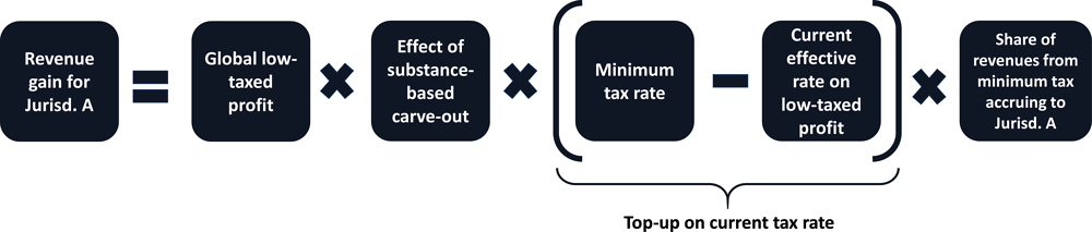
Note: The starting point to compute the revenue effects of Pillar Two is to assess the amount of low-taxed profit of MNEs (i.e. profit taxed at a rate below the potential minimum rate level). The effect of a potential formulaic substance-based carve-out is to exclude a fraction of these low-taxed profits from the scope of Pillar Two. Then, Pillar Two operates as a ‘top-up’ to bring the effective tax rate on the low-taxed profits in scope up to the level of the minimum rate (parenthesis of the formula). Finally, the share of Pillar Two revenue gains accruing to each jurisdiction is determined based on assumptions on the functioning of Pillar Two that are described in this chapter.
Source: OECD Secretariat
181. Consistent with the Pillar Two Blueprint report, the approach in this chapter is to assume that MNEs’ low-taxed profits would generally be subject to a top-up tax in the jurisdiction of the ultimate parent entity of the MNE group under the income inclusion rule. The switch-over rule is not explicitly modelled in this chapter, but would implicitly contribute to the application of the income inclusion rule. Similarly, it is challenging to determine, based on the design of the subject to tax rule and the available data, what impact that rule would have on a jurisdiction’s tax base. Given these challenges, the impact of the subject to tax rule has not been modelled in this chapter.
182. In the stylised scenarios considered for the purpose of modelling in this chapter, certain ultimate parent jurisdictions would not necessarily introduce an income inclusion rule (e.g. jurisdictions that do not have a corporate tax system today). The low-taxed profits of MNEs with an ultimate parent in these jurisdictions are assumed to face the top-up tax in other jurisdictions, in proportion to the distribution of their economic activity across these other jurisdictions. This assumption is a proxy for the transaction-based approach envisaged under the undertaxed payments rule, with the idea that transactions subject to this rule are likely to originate in jurisdictions where the MNE group considered engages in economic activity. This assumption can also be seen as a possible proxy for situations where the jurisdiction of an intermediate parent would apply the income inclusion rule, as envisaged in the Pillar Two Blueprint report, assuming that the location of these intermediate parents (on which no data are available in most jurisdictions) is broadly aligned with the location of economic activity.
183. Another important Pillar Two design question is the degree of “blending” (i.e. the level of aggregation at which the effective tax rate would be computed and the minimum rate applied). While no decision has been taken by the Inclusive Framework yet, it is assumed in this chapter that Pillar Two would entail jurisdictional blending in line with the Pillar Two Blueprint report. This would imply that the ETR of an MNE would be computed by aggregating taxes paid and profits at the jurisdiction level. This ETR would then be compared to the minimum tax rate.
184. Other Pillar Two design and parameter choices will also influence the revenue effects of Pillar Two. A key parameter is the potential minimum tax rate – in this area, several possibilities are illustratively explored in this chapter. Other questions include the definition of the tax base (including questions related to adjustments for permanent and temporary book-tax differences), the definition of taxes covered in the computation of the ETR, the existence and design of a potential loss carry-forward mechanism, and the existence and scope of potential ‘carve-outs’ based on substantive activities and/or for certain sectors or in relation to MNE size. Consistent with the Pillar Two Blueprint report, MNEs with a global turnover below EUR 750 million (i.e. the Country-by-Country Reporting threshold) are assumed not to be in the scope of Pillar Two in the estimates in this chapter. The implications of a potential formulaic substance-based carve-out are illustratively modelled in this chapter, while no sectoral carve-outs are considered in the estimates due to data limitations. Finally, the effect of a potential loss carry-forward mechanism is not taken into account, due to lack of time series data on MNE profit across jurisdictions,3 while the inclusion of such a mechanism could reduce potential revenue gains from Pillar Two.
185. While no decision has been taken by the Inclusive Framework yet, the estimates in this chapter are based on the illustrative assumption that the US GILTI regime would “co-exist” with Pillar Two. Reflecting this, the estimates presented in this chapter generally exclude the potential revenue gains related to US MNEs on the basis that they would remain subject to GILTI and not subject to Pillar Two rules. This means that in the tables and figures presenting estimates of Pillar Two revenue gains in this chapter, gains related to US MNEs (including both direct gains from the minimum tax and indirect gains from reduced profit shifting or ETR increases) are generally excluded. This is indicated in the subtitles and reading notes of these tables or figures. Other tables containing intermediate data or results not directly representing Pillar Two gains (e.g. profit matrix at an aggregated level) generally include data relative to US MNEs, as indicated in the notes of these tables. Revenue gains related to US MNEs are discussed in Section 3.8, based on the ex ante estimates of GILTI revenue gains from the US Joint Committee on Taxation (JCT).
186. In considering potential behavioural reactions, a series of four stylised scenarios are modelled. These scenarios are summarised in Figure 3.2. These scenarios and the strategy to quantify their revenue implications are described in more detail in the following sections.
Scenario 1, which is the starting point for the estimates, is a “static” scenario. In this scenario, potential behavioural reactions of MNEs and governments to the introduction of Pillar Two are not taken into account, and Pillar Two is modelled in isolation, in the sense that its potential interaction with Pillar One is not taken into account.
Scenario 2 takes into account the interaction between Pillar One and Pillar Two. In this scenario, Pillar Two is assumed to apply on profit after the reallocation implied by Amount A of Pillar One, as modelled in Chapter 2, based on illustrative assumptions on Pillar One design and parameters. Alternative results ignoring this interaction but accounting for the reactions of MNEs and governments modelled in Scenarios 3 and 4 are presented in Annex 3.B.
Scenario 3 builds on Scenario 2 by adding the assumption that MNEs’ profit shifting intensity would be reduced by Pillar Two. This is because Pillar Two would reduce tax rate differentials between jurisdictions, which are a primary driver of profit shifting. This reduction in profit shifting is assessed based on stylised modelling assumptions that are discussed further in Section 3.6.
Scenario 4 builds on Scenario 3 by adding the assumption that certain jurisdictions would change certain tax rules/rates to increase the ETR on MNE profit that is currently taxed below the minimum rate in their jurisdiction. The rationale for this reaction is that it could allow the jurisdictions increasing their ETR to collect a greater share of global tax revenues, while having only a generally limited effect on the overall tax payments of MNE groups (as discussed below, this effect would depend on the design of Pillar Two and notably on the potential inclusion of a formulaic substance-based carve-out, as well as the potential co-existence of the US GILTI regime with Pillar Two).

Note: Other behavioural reactions to Pillar Two are also possible, but they are not modelled in this chapter. These non-modelled reactions include for example changes in MNE ‘real’ investment location (with potential implications for CIT revenues but also for revenues from other tax bases) as well as policy changes in jurisdictions with an average ETR above the minimum rate. These potential reactions are discussed in Chapter 4.
Source: OECD Secretariat.
187. The timing of MNEs’ and governments’ reactions considered in Scenarios 3 and 4 is uncertain, raising the question of the order in which they should be considered in the analysis. It is possible that MNEs’ profit shifting strategies would be adjusted faster and with more precision than governments’ corporate tax systems. Indeed, the latter may involve a multiplicity of interconnected statutory provisions, all having different effects on the tax position of different firms, and any adjustments could require lengthy law-making processes to take place. This justifies considering MNE reactions first (in Scenario 3) and government reactions second (in Scenario 4). However, given the scenarios and assumptions considered in this chapter, reversing this order (i.e. considering government reactions first and MNE reactions second) would have virtually no (or at most a quantitatively very small) effect on the final results. The reason is that the government reactions considered in this chapter do not significantly affect the profit shifting incentives of MNEs, since they do not change significantly the overall amount of taxes paid by MNEs (they only change where taxes are paid).4 As a result, MNEs’ reactions are not expected to depend substantially on whether they are considered before or after government reactions, at least under the stylised scenarios considered in this chapter.
188. The four stylised scenarios presented in this chapter do not aim to cover the full universe of possible reactions, but to illustrate the implications of some of the most widely expected reactions to Pillar Two. The reactions considered have been selected based on earlier discussions with jurisdiction representatives, academics, private sector representatives and other international organisations. Other potential reactions are not modelled in this chapter, including MNEs modifying their ‘real’ investment behaviour (as opposed to profit shifting intensity), MNEs modifying their profit shifting strategies in more complex ways than envisaged in this chapter, and governments from higher-tax jurisdictions (i.e. with average ETRs above the potential minimum rate under Pillar Two) reacting to the introduction of Pillar Two by changing their tax rules or rates:
On MNEs’ real investment behaviour, the OECD Secretariat estimates suggest that Pillar Two would only result in limited effects on forward-looking average ETRs at the global level and across most jurisdictions (Chapter 4). This would indicate that the scale of investment effects would generally be limited (in addition, these effects could be offset, partly or fully, by the indirect effects discussed in Chapter 4), providing justification for the assumption not to take these effects into account in this chapter. An important exception is that jurisdictions that currently have an ETR below the potential minimum rate could face significant ETR increases. This would affect MNE investment into these low-tax jurisdictions, while possibly benefitting higher-tax jurisdictions where some investment may be redirected. In turn, this would reduce corporate tax revenues in these low-tax jurisdictions, as well as revenues from other tax bases (e.g. personal income tax, value added tax). These effects are not modelled in this chapter.
On MNE profit shifting strategies, the modelling in this chapter is based on simplified assumptions described below relating to profit shifting intensity to tax rate differentials between jurisdictions. In practice, MNE profit shifting schemes are often complex and largely firm-specific. The exact way in which these schemes could be modified in reaction to Pillar Two may differ from these simplified assumptions, which would influence final outcomes, but this is impossible to model with precision, as further discussed below.
On the policy reaction of “higher-tax” jurisdictions (i.e. jurisdictions with an average ETR above the potential minimum rate), the expected reaction is ambiguous and therefore difficult to anticipate with certainty, as further discussed in Chapter 4. In theory, the introduction of a minimum rate could strengthen or weaken tax competition depending on the assumptions considered (Keen and Konrad, 2013[3]).5 An empirical study on the 2004 introduction of a minimum tax rate at the municipal level in Germany suggests that, on average, it led to municipalities with rates above the minimum significantly increasing their rates (von Schwerin and Buettner, 2016[4]), However, it is not clear to what extent these results can be generalised from a national to a global context.
189. The simplified approach followed in this chapter is to identify jurisdictions where the average (backward-looking) ETR on MNE profit is below the potential minimum tax rate. All MNE profit in these jurisdictions is assumed to be taxed at this average ETR (due to lack of available firm-level data on ETRs in most jurisdictions), and therefore – after application of a potential formulaic substance-based carve-out – to face a top-up tax up to the level of the minimum tax.
190. This is a simplification in the sense that it does not take into account that (i) some MNE profit may be subject to a higher ETR than the minimum rate in low-tax jurisdictions (pockets of high-taxed profits) and (ii) some MNE profit may be subject to a lower ETR than the minimum rate in higher-tax jurisdictions (pockets of low-taxed profits). Pockets of low-taxed profit are further discussed in Box 3.1 below and are taken into account in the uncertainty ranges around the results. Pockets of high-taxed profit seem likely to be less common than pockets of low-taxed profit and the effect of their omission is a priori ambiguous (because taking pockets of high-taxed profit into account would reduce the estimated amount of profit subject to Pillar Two in low-tax jurisdictions, but also reduce the average ETR on profit subject to Pillar Two in these jurisdictions). Due to data limitations, the approach also overlooks the fact that some foreign profit may already be taxed at the parent level via controlled foreign company (CFC) rules and withholding taxes. This would reduce Pillar Two gains.
191. This modelling approach requires data on the location of profit as well as data on ETRs. The source of data on profit is described in the next section, while data on ETRs are presented in the following one. The modelling of the implications of a potential formulaic substance-based carve-out is described afterwards.
3.4.1. Data source on profit location: The “profit matrix”
192. As in Chapter 2, the analysis in this chapter relies on the “profit matrix”, which combines data from different sources on the location of MNE profit (see stylised illustration in Figure 3.3 and detailed description in Chapter 5).

Note: Aggregate CbCR data are used to fill columns of the profit matrix (e.g. profit of French MNEs across jurisdictions). ORBIS unconsolidated account data are used to fill rows of the profit matrix (i.e. MNE profit in France, split across ultimate parent jurisdictions). These two sources are used only where available, and in the case of ORBIS, where data coverage is sufficiently good. Other cells in the profit matrix are filled with extrapolations based on macroeconomic data, including FDI data.
Source: OECD Secretariat.
193. The profit matrix draws on three main sources of data, presented below in descending order of preference:
1) Anonymised and aggregated data from Country-by-Country Reports (CbCRs), across 25 jurisdictions of ultimate parent (see list in Annex 5.A of Chapter 5);6
2) ORBIS unconsolidated account data in 24 jurisdictions of affiliate with good ORBIS coverage (see list in Annex 5.A of Chapter 5);
3) Extrapolations based on macroeconomic data (e.g. FDI data) in other cells.
194. Wherever possible, the data in the profit matrix (and in the tangible assets and payroll matrices described below) focus on MNE sub-groups with positive profits (i.e. entities belonging to an MNE group that is reporting an overall profit in the jurisdiction considered), rather than all MNE sub-groups (i.e. profit-making and loss-making sub-groups). Indeed, only MNE sub-groups with positive profits potentially face additional taxes under Pillar Two, while loss-making sub-groups generally do not pay corporate income tax. Subtracting the losses of loss-making MNE sub-groups when computing total profit in a jurisdiction could therefore lead to an underestimation of the amount of profit that could be subject to Pillar Two.
195. Still, a limitation of the approach is that the effect of a loss carry-forward mechanism under Pillar Two is not taken into account in the estimates. Such a mechanism could reduce revenue gains from Pillar Two in situations where an MNE sub-group in a low-tax jurisdiction makes a (low-taxed) profit and can use its past losses in that jurisdiction to offset it partly or fully. Estimating with precision the effect of the loss carry-forward mechanism would require firm-level information on the profitability of MNE sub-groups over several successive years. This information is not available to the OECD Secretariat in most jurisdictions.7 In practice, the effect of the loss-carry forward mechanism on Pillar Two revenue gains will depend on how frequently MNE sub-groups in low-tax jurisdictions switch from being loss-making to being profitable. This may depend on the economic situation – for example, the COVID-19 crisis is likely to make losses more frequent – but also on profit shifting and loss shifting behaviour by MNEs. For example, even taking into account a carry-forward mechanism under Pillar Two, it may still be more beneficial for MNEs to incur losses in higher-tax than in low-tax jurisdictions, as these losses can be used to offset future profits at a higher rate in higher-tax jurisdictions.
196. The profit matrix – at a relatively high level of aggregation – is displayed in Table 3.1. The full methodology underlying the construction of the profit matrix is presented in detail in Chapter 5. Chapter 5 also contains detailed information on the data sources used in the profit matrix, including a discussion of the caveats around their use. In addition, Chapter 5 displays a more disaggregated version of the profit matrix (i.e. with more detailed jurisdiction groups than in Table 3.1), as well as information on the relative importance of the different data sources underlying the matrix. Finally, Chapter 5 contains the results of the extensive benchmarking that was undertaken to assess the quality of the data and its consistency across sources.
3.4.2. Data sources on effective tax rates (ETRs)
197. The relevant ETR to assess if an MNE has low-taxed profit in a jurisdiction and would be subject to Pillar Two will be computed at the level of each MNE sub-group in each jurisdiction (assuming that Pillar Two would involve jurisdictional blending). Estimating with precision the effect of Pillar Two would therefore require data on ETRs at that level. However, the data are not available to the OECD Secretariat in most jurisdictions, and the approach therefore relies on average ETRs computed from aggregated data.
198. The average ETR on MNE profit in a jurisdiction is measured as the median estimate obtained across the three following data sources:
Data from Tørsløv et al. (2018[5]). These data, themselves based on a combination of sources and assumptions, focus on the ETR on the profit of foreign-owned MNEs across a range of jurisdictions in 2015. The underlying data generally does not distinguish between profit-making and loss-making MNE sub-groups and can thus lead to higher measures of ETR than data that would focus only on profit-making sub-groups.8
Data from the US Bureau of Economic Analysis (BEA) on US MNEs. In an annual report on the global activity of US MNEs, the BEA provides information on foreign taxes paid by affiliates of US MNEs across a set of jurisdictions. In each of these jurisdictions, the average ETR of US MNEs is computed by dividing foreign taxes paid by “profit-type return”, which is a measure of profit included in the BEA data that aims to approximate profit before tax and excludes various sources of financial income. To reduce the impact of potential volatility in the data, the ETR used in this chapter is computed as the average ETR over several years (2013-16), i.e. the sum of taxes paid in a jurisdiction over the period divided by the sum of profit-type returns in this jurisdiction over the same period.9 As with the data from Tørsløv et al. (2018[5]), the BEA data aggregates data relative to profit-making and loss-making MNE sub-groups, which leads to higher ETRs than when focusing only on profit-making sub-groups.
Data from anonymised and aggregated CbCR reports. The anonymised and aggregated CbCRs from 25 jurisdictions of ultimate parent (see list in Annex 5.A of Chapter 5) have been used to compute average ETRs by jurisdiction of affiliate. The ETR in a given jurisdiction of affiliate is computed as the total taxes paid by foreign-owned MNEs (on an accrual basis) over total profit of foreign-owned MNEs, focusing only on profit-making sub-groups (contrary to the other two sources). Extreme outliers are eliminated (e.g. ETRs above 100%) and jurisdictions covered in the data of fewer than three ultimate parent jurisdictions are excluded. An important caveat is that due to potential inclusion of intracompany dividends in profit reported in CbCRs, ETRs may be underestimated, especially in jurisdictions with a large presence of parent companies (OECD, 2020[6]).
199. None of these three measures of ETRs is subject to the issue of profit double counting pointed out by Blouin and Robinson (2019[7]) (see also discussion in Clausing (2020[8])). In addition, using the median value across the three measures reduces the potential impact of limitations of individual data sources on the final revenue estimates (e.g. limitations related to the potential inclusion of dividends in CbCR data, which could lead to overestimating Pillar Two gains, or to the fact that data from Tørsløv et al. (2018[5]) and BEA data include loss-making sub-groups, which could lead to underestimating Pillar Two gains). A robustness analysis excluding CbCR data from the calculation and relying only on the average of the other two sources suggests that it could lead to lower estimates of Pillar Two gains, but without changing the broad order of magnitude of the results (see Annex 3.D).
200. All three data sources are available jointly for 42 jurisdictions representing 86% of world GDP (Table 3.2). At least one of the three data sources is available for another 99 jurisdictions, representing another 12% of world GDP. For the other 81 jurisdictions considered in the analysis, which are mainly lower income jurisdictions that together represent only 1% of world GDP, none of these three sources are available and the ETR is assumed to correspond to the statutory CIT rate, sourced from the OECD Corporate Tax Statistics (OECD, 2020[9]), complemented with other sources.10 This is a conservative assumption since ETRs are generally lower than statutory rates. However, the impact of this assumption on the global estimates is likely to be marginal as less than 1% of total MNE profit is found to be located in these jurisdictions.
3.4.3. Global low-taxed profit and global revenue gains (before carve-out)
201. Based on the profit matrix and the ETR data described above, the global amount of low-taxed profit (i.e. profit taxed below a potential minimum rate) is presented in Table 3.3 for an illustrative range of potential minimum rates. Estimated global gains from Pillar Two are then obtained by topping up the tax rate on the low-taxed profits up to the level of the minimum rate.11 A ±10% uncertainty range around the point estimates is applied to take into account data uncertainty. The results, which are presented in Table 3.3, correspond to the revenue gains in Scenario 1 (i.e. in a static scenario that does not take into account the interaction with Pillar One, nor behavioural reactions by MNEs and governments) with no formulaic substance-based carve-out. Consistent with the assumptions on GILTI discussed above, the table excludes the low-taxed profit of US MNEs and the corresponding revenue gains (revenue gains from GILTI are discussed in Section 3.8).
202. These estimates do not take into account potential gains related to pockets of low-taxed profit in higher-tax jurisdictions (i.e. jurisdictions with an average ETR above the minimum rate). These pockets, while difficult to assess with the available data, may be substantial, as discussed in Box 3.1. Not taking them into account could lead to significantly underestimating the revenue gains from Pillar Two. In light of this, the upper bound of the uncertainty ranges surrounding the estimates of the direct gains from Pillar Two in Scenario 1 is increased by 50% (last row in Table 3.3). Such an increase in revenue gains would correspond to a situation where pockets of low-taxed profit would represent close to 10% of total profit in higher-tax jurisdictions (Box 3.1). The lower bound of the uncertainty ranges is not changed and therefore assumes conservatively no revenue gains from these pockets. In scenarios with a formulaic substance-based carve-out (discussed below), the uncertainty around these pockets is reduced in proportion to the share of carved-out profit in higher-tax jurisdictions.12
203. The estimates in Table 3.3 are broadly consistent with recent estimates by the Oxford University Centre for Business Taxation (Devereux et al., 2020[10]). Assuming a 10% minimum tax rate, no formulaic substance-based carve-out, and including MNEs with an ultimate parent in the United States, they assess that global Pillar 2 revenue gains in a static scenario could reach USD 20 billion (1.1% of global CIT revenues) in an approach excluding pockets of low-taxed profit in higher-tax jurisdictions, or USD 32 billion (1.8% of global CIT revenues) in an approach including them.13 This is higher than the estimates with corresponding assumptions in Table 3.3 (i.e. estimated gains of 0.8%-1.0% of CIT revenues excluding pockets of low-taxed profit, and 0.8%-1.5% of CIT revenues including them) but the difference is likely explained in large part by the fact that the estimates in Table 3.3 exclude MNEs with an ultimate parent in the United States, while the estimates by Devereux et al. (2020[10]) include them.
The methodological approach in this chapter focuses on low-taxed profit in low-tax jurisdictions (i.e. jurisdictions with an average ETR below the minimum rate) and overlooks potential “pockets” of low-taxed profit in higher-tax jurisdictions. It is impossible with the available data to assess with precision the size of these pockets. Indeed, this would require detailed data on profit and taxes paid at the firm level. The limited sources available to the OECD Secretariat (i.e. ORBIS database in jurisdictions with good data coverage, and confidential information from national sources collected via jurisdiction delegates to the OECD Working Party No. 2 on Tax Policy Analysis and Tax Statistics) suggest that the shape of the distribution of MNE ETRs varies widely across the jurisdictions covered. In addition, while these sources suggest that these pockets can be substantial, they give inconsistent signals on the shape of the ETR distribution in certain jurisdictions, suggesting potential differences in the definition of ETR considered (e.g. due to different accounting methods) or data quality issues. In particular, the available data may not necessarily allow for the measurement of ETRs in a way that would be consistent with the approach used in the context of Pillar Two.
An estimate based on stylised and illustrative assumptions on the distribution of ETRs across firms suggest that low-taxed profit (i.e. profit taxed at an ETR below the minimum rate) could represent about 8% of total profit in higher-tax jurisdictions, assuming a 12.5% minimum tax rate. This estimate is based on a methodology developed by the European Commission and applied to the data underlying this chapter.1 Given the uncertainty around the actual distribution of ETRs, this estimate should be seen as an illustrative order of magnitude rather than a precise point estimate.
The total amount of profit in higher-tax jurisdictions (i.e. jurisdictions with an average ETR above the minimum rate) is about USD 3 400 billion, if one assumes illustratively a 12.5% minimum rate (for comparability with other results in this chapter, this excludes US MNEs). If, out of this total, one would assume – for the purpose of illustration – that 5-10% of profit is taxed below the minimum rate (consistent with the 8% estimate above), this would represent USD 170-340 billion of additional low-taxed profit globally, which would come on top of the USD 604 billion of profit in low-tax jurisdictions already considered in the analysis (see Table 3.3). This could imply an increase in estimated revenue gains (in a static scenario) by about 30-60%.2
As further discussed below, a formulaic substance-based carve-out could reduce the size of these pockets. Indeed, under the range of carve-out design and parameter options considered in this chapter, about 10-35% of profit in higher-tax jurisdictions could be carved out (Table 3.5), potentially reducing the size of these pockets by that amount.
← 1. The assumption is that ETRs in each jurisdiction follow a bilinear distribution between zero and the statutory rate, centred around the average ETR. This amounts to assuming that a fraction of profit is uniformly distributed between zero and the average ETR, and the rest is uniformly distributed between the average ETR and the statutory rate. The share of profit in each group is determined in a way that ensures that the average of ETRs across the distribution corresponds to the average ETR in the jurisdiction.
← 2. This assumes implicitly that the current average ETR in these pockets of low-taxed profit (which is not observed), is the same as the average ETR in low-tax jurisdictions. A different assumption would give different estimates.
3.4.4. Modelling the implications of a formulaic substance-based carve-out
General approach to model a formulaic substance-based carve-out
204. The Pillar Two Blueprint report envisages that the GloBE rules (IIR and UTPR) could include a formulaic substance-based carve-out based on a fixed percentage of payroll plus a fixed percentage of depreciation expenses on a broad range of tangible assets (OECD, 2020[1]). These two percentages could be identical or different. The illustrative results presented in this chapter assume identical percentages.
205. For example, if one assumes illustratively a 10% carve-out percentage (or "mark-up”) for both payroll and depreciation expenses, the GloBE rules would only apply to a given MNE sub-group in a given jurisdiction on the profits that exceed 10% of the sum of payroll plus depreciation expenses of that MNE sub-group in that jurisdiction. For example, if the profit of the sub-group is 100, its payroll 150 and its depreciation expenses 50, the profit on which Pillar Two applies would be 100-10%*(150+50)=80.
206. On this profit, Pillar Two would apply, as before, by topping-up the average ETR paid by the MNE sub-group in that jurisdiction up to the level of the agreed minimum tax rate. The Inclusive Framework will define at a later stage the exact rules to calculate this ETR in the presence of a carve-out, and in particular whether an MNE group that claims the benefit of the carve-out should be required to make a corresponding and proportional adjustment to the covered taxes. For example, if before the application of the carve-out a taxpayer has EUR 100 of profit and EUR 20 of covered taxes, the ETR in absence of carve-out is 20% (EUR 20 divided by EUR 100). If the carve-out reduces the taxpayer’s profit to EUR 80, then the ETR for the purposes of the GloBE rules could be either (i) EUR 20 of covered taxes divided by EUR 80 of profit (i.e. 25%) if the MNE is not required to make an adjustment to the covered taxes, or (ii) EUR 16 of covered taxes divided by EUR 80 of profit (i.e. 20%) if the MNE is required to make an adjustment to the covered taxes that would be corresponding and proportional to the effect of the carve-out on profit. The approach modelled in this chapter is the second, since the modelling relies on the same ETRs in the scenarios with and without the carve-out. This reflects that modelling the situation without adjustment would be difficult with the available data, and does not prejudge future decisions by the Inclusive Framework on this question. Since the first approach (i.e. without adjustment) would result in higher ETRs than the second approach, it would lead to lower revenue gains (for a given level of the minimum rate and the carve-out percentage).
207. Modelling with precision the impact of a carve-out would require firm-level information on tangible assets depreciation and payroll across all jurisdictions. Sufficiently detailed firm-level data at the unconsolidated level is available in the ORBIS database with good coverage for only 18 to 24 jurisdictions depending on the variable considered (see list in Annex 5.A of Chapter 5).14 In these jurisdictions, the share of carved-out profit is computed directly with ORBIS data, at the level of each MNE sub-group, as discussed below. In the other jurisdictions, the approach relies on more aggregate data, in combination with an analysis based on ORBIS data on the average relationship between firm-level and aggregate data, which is also described below.
208. The approach in this chapter is to estimate the share of carved-out profit in all jurisdictions, even those with average ETRs above the minimum rate. This offers the benefit of helping to gauge the effect of the carve-out on potential pockets of low-taxed profit in these jurisdictions. For practical reasons, the payroll carve-out and the depreciation carve-out are modelled separately, and their effects are summed to obtain the effect of a combined carve-out.15 This represents an approximation compared to the actual effect of a combined carve-out, because it could lead to some ‘double counting’ of carve-out effects in cases where the sum of the amounts carved out under each carve-out taken individually would exceed the total profit of the MNE sub-group considered.16 Computations based on ORBIS firm-level data suggest that this double counting is not quantitatively significant under the carve-out percentages considered in this chapter, as it leads to an overestimation of the effect of the carve-out by less than 4% on average across jurisdictions.
209. The coverage of depreciation expenses in ORBIS is less extensive than the coverage of tangible assets. In addition, depreciation is generally aggregated with amortisation of intangible assets. In aggregate data as well, the level of tangible assets is generally better covered than depreciation expenses. Against this background, the approach to approximate depreciation expenses is to use data on tangible assets combined with an assumption on the average depreciation rate. Evidence from the available data from the US BEA and the ORBIS database suggests that the average depreciation rate of tangible assets (i.e. property, plant and equipment) is about 5-10%,17 and this percentage is conservatively assumed to be 10% in the estimates of this chapter.
The aggregate data in the tangible assets and payroll matrices
210. Aggregate data on the location of MNE tangible assets and payroll across jurisdictions are based on a ‘tangible assets matrix’ and a ‘payroll matrix’ that combine various data sources and extrapolations, in the same spirit as the profit matrix. These data sources and methodology underlying these two matrices, as well as extensive benchmarking and checks to assess their quality are presented in Chapter 5. These matrices are presented at an aggregate level in Table 3.4.
211. An important caveat to the analysis of carve-outs is that the definition of tangible assets and payroll in the data underlying the matrices may not necessarily match the exact definitions of the variables considered for a formulaic substance-based carve-out. The tangible assets matrix focuses on property, plant and equipment, net of accumulated depreciation, while the payroll matrix focuses on expenditures for salaries and wages, including bonuses, social contributions and other employee benefits (see Chapter 5). While this is broadly consistent with the variables considered for a carve-out, which are described in the Pillar Two Blueprint report, there may be differences related, for example, to the treatment of land or subcontracted labour expenses, which, depending on the exact definition of the carve-out, could affect the accuracy of the estimates.
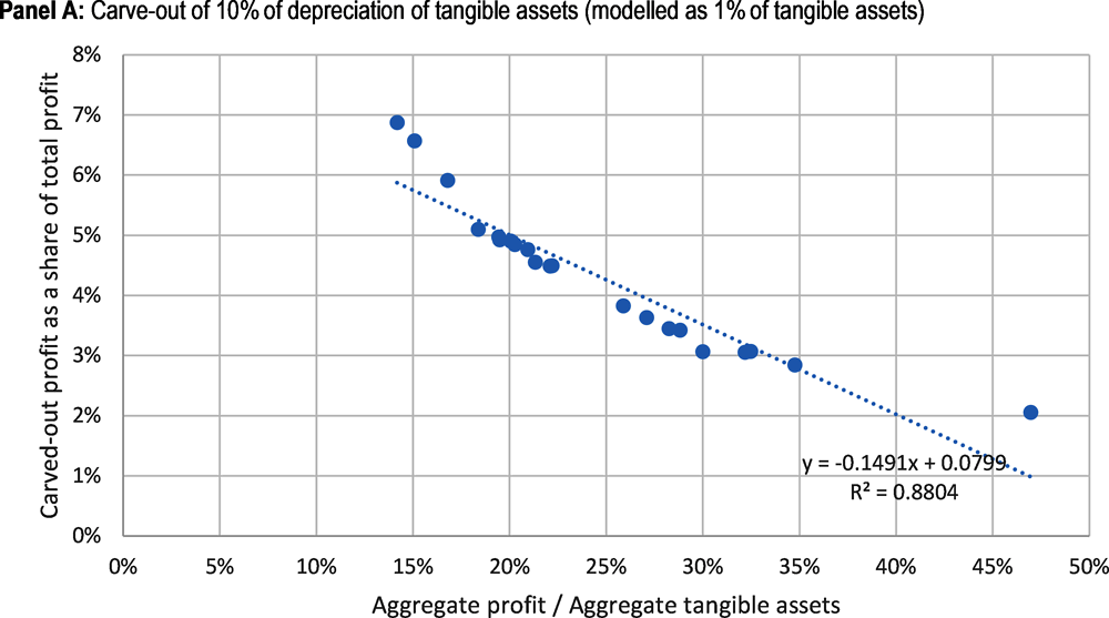

Note: Each dot corresponds to one jurisdiction. Non-carved-out profit is computed for each MNE sub-group as profit before tax in excess of 1% of tangible assets (panel A) or 10% of payroll (Panel B). These figures focus on all profit-making MNE sub-groups in the jurisdictions considered, regardless of their ETR. Loss-making MNE sub-groups in the jurisdiction are not included. The sample consists of jurisdictions with relatively good coverage of unconsolidated accounts in ORBIS on both foreign and domestic MNE entities for the variables considered (tangible assets in Panel A, payroll in Panel B), see list in Annex 5.A of Chapter 5.
Source: OECD Secretariat calculations based on ORBIS data.
Average relationship between firm-level estimates of carved-out profit and aggregate data on profitability
212. The share of profit that would be carved out for a range of illustrative carve-out percentages is computed with precision, at the level of each MNE sub-group, with ORBIS unconsolidated firm-level data across the jurisdictions with good ORBIS coverage on both foreign and domestic MNE entities (see list in Annex 5.A of Chapter 5). ORBIS financial and ownership data used for this analysis have been cleaned extensively using OECD Secretariat expertise from past projects, as described in Annex 5.B of Chapter 5.
213. As discussed above, the effect of the payroll and depreciation components of the carve-out are computed separately, and then summed. The results on the share of carved-out profit for each component are presented in Figure 3.4 for an illustrative value of the carve-out percentage (10%) across the jurisdictions with good ORBIS coverage (each dot corresponding to one jurisdiction).
214. The results in Figure 3.4 suggest that the share of carved-out profit in a jurisdiction is relatively well correlated with the aggregate profitability ratio at the jurisdiction level (profit to tangible assets or profit to payroll, depending on the panel considered). For example, results in Panel A suggest that the share of carved-out profit with a 10% carve-out on tangible assets depreciation is well correlated with the ratio of aggregate profit to aggregate tangible assets at the jurisdiction level. This average relationship is used to extrapolate the share of carved-out profit in jurisdictions with poor ORBIS coverage, based on aggregate data from the profit, tangible assets and payroll matrices. The approach is very similar to the one employed on the assessment of Pillar One to assess the share of profit that is residual based on aggregate profit and turnover (see Chapter 2). For example, in the case of tangible assets, the relationship, which is estimated over the jurisdictions with good ORBIS coverage, is the following:
215. This relationship is estimated for each carve-out percentage considered in the analysis (5%, 10%, 15% and 20%). There is no theoretical reason why this relationship should be linear, but in practice a linear relationship seems to offer a reasonably good fit and the number of observations is insufficient to consider more complex specifications.18
216. The estimation for a 10% carve-out percentage is presented in Figure 3.4 for depreciation (Panel A) and payroll (Panel B). The correlation for the other percentages considered in the analysis is broadly similar to the correlation observed with a 10% percentage, but the coefficients and differ. In general, a higher carve-out percentage would lead to a higher since it would increase the share of carved-out profit, while the differences in depend on the shape of the distribution of profit, tangible assets, and payroll across jurisdictions. The results presented in the following sections are based on the specific coefficients and corresponding to the carve-out percentage considered (e.g. results for a 5% carve-out percentage are based on the and estimated for that percentage).
Share of carved-out profit across jurisdiction groups
217. Based on this methodology, the share of carved-out profit in each cell of the profit matrix is computed for a range of carve-out percentages. The results are presented (at a high level of aggregation) in Table 3.5. For example, assuming a 10% carve-out percentage, 15% of global profit would be carved out. This share is much lower in investment hubs (2%) than in other jurisdictions groups (16-19%) reflecting that a relatively high share of MNE profit is located in investments hubs compared to their share of tangible assets and payroll. Among investment hubs, the share of carved-out profit tends to be even lower among zero-tax jurisdictions (less than 1%) than non-zero-tax jurisdictions (2%).
218. As Pillar Two operates by allowing jurisdictions to ‘tax back’ low-taxed profit that is located in other jurisdictions, the share of carved-out profit in a jurisdiction influences Pillar Two gains in other jurisdictions. In particular, the fact that the share of carved-out profit in investment hubs is relatively small (while an important share of global low-taxed profit is located in investment hubs) implies that the effect of the formulaic substance-based carve-out considered in this chapter on Pillar Two revenue gains across jurisdictions is limited, as can be seen in the next section.
Effect of formulaic substance-based carve-out on Pillar Two gains under Scenario 1
219. The effect of Pillar Two in a static scenario (i.e. Scenario 1) with a formulaic substance-based carve-out is computed in the same way as before the carve-out, with the difference that the amount of profit on which Pillar Two is applied is non-carved-out profit, instead of total profit. The data on ETRs are the same as in the no-carve-out case, which, as discussed above, is consistent with the assumption that MNEs would be required to make an adjustment to the covered taxes that would be corresponding and proportional to the effect of the carve-out on profit.
220. The results, which are presented in Table 3.6, suggest that the effect of a formulaic substance-based carve-out on Pillar Two revenue gains is relatively small, especially when pockets of low-tax profit in higher-tax jurisdictions are not considered. For example, in the case of a 10% carve-out, the estimated Pillar Two gains would be reduced by about 3%. When taking into account the potential effect of the carve-out on pockets of low-taxed profit in the uncertainty ranges (last row in Table 3.6), the upper bound of the ranges is reduced significantly by the carve-outs. This reflects that profit in these pockets is likely to benefit more from a formulaic substance-based carve-out than profits in jurisdictions with low average ETRs, where less economic activity may generally be located.19
3.4.5. Methodology to estimate jurisdiction-level revenue gains
221. Revenue gains at the jurisdiction level and, in turn, for jurisdiction groups are derived using the following stylised modelling assumptions, also summarised in Figure 3.5, which do not pre-judge jurisdictions’ actual implementation decisions:
Group 1: Jurisdictions with an average ETR above the minimum rate. These jurisdictions are assumed to implement an income inclusion rule (IIR), in the sense that they would apply a top-up tax to ensure that the profit of MNE entities (blended at the jurisdictional level) with an ultimate parent in their jurisdiction is taxed at least at the minimum rate.20 They are also assumed to implement an undertaxed payments rule (UTPR). Consistent with the Pillar Two Blueprint report, the IIR is assumed to apply in priority to the UTPR.21
Group 2: Jurisdictions with a zero corporate tax rate. For the purposes of modelling, these jurisdictions are assumed not to introduce an IIR nor a UTPR, as it would also require introducing a corporate income tax (CIT) system, which many of these jurisdictions do not have. As a result, the low-taxed profit of MNE entities with an ultimate parent in these jurisdictions would not be taxed by these jurisdictions (since they would not introduce an IIR). If an intermediate-level parent (i.e. a parent entity that is not the ultimate parent) in the MNE group is located in a jurisdiction introducing an IIR, this low-taxed profit would be taxed by the jurisdiction of this intermediate parent (if there are several intermediate parents in this case, the highest one in the ownership chain would have priority according to the top-down principle described in the Pillar Two Blueprint report). If the low-taxed profit is not in scope of an applicable IIR (e.g. if there is no intermediate-level parent, or if intermediate parent jurisdictions are not introducing an IIR, or if the ultimate parent jurisdiction is low tax), the low-taxed profit could be taxed under the UTPR of a jurisdiction introducing a UTPR and from which intra-group payments originate.
In practice, it is difficult with the available data to model these rules with precision, as little information is available on the location of intermediate parents and transaction origins. Reflecting this, it is assumed for the purposes of modelling in this chapter that the profits of MNEs with an ultimate parent in Group 2 would be subject to a top-up tax imposed by other jurisdictions, in proportion to the amount of economic activity located in these jurisdictions (as a proxy for the location of intermediate parents in the case of IIR, and of the transactions-based nature of the UTPR).
Economic activity is proxied by MNE turnover, sourced from the “turnover matrix” described in Chapter 5.22,23 Results are broadly robust to using tangible assets or payroll instead of turnover as a proxy (see Annex 3.C). When economic activity is located in a jurisdiction that does not implement an IIR nor a UTPR (e.g. a jurisdiction in Group 2), the corresponding low-taxed profit is assumed not to be subject to the top-up tax. However, this represents a relatively small fraction of total low-taxed profit under the assumptions considered in this chapter.
Group 3: Jurisdictions with an average ETR below the minimum rate, but greater than zero. Among jurisdictions in Group 3, for the purposes of this modelling scenario, half are assumed to implement an IIR and a UTPR (as jurisdictions in Group 1), and the other half are assumed not to implement them (as jurisdictions in Group 2). One reason why it is likely that not all jurisdictions in this group would implement an IIR and a UTPR is that some of these jurisdictions may decide that imposing a minimum tax rate on foreign profits could seem inconsistent with maintaining an average ETR below this minimum rate on local profit. As a result, this choice may be linked to choices relative to other tax policy parameters, and more specifically whether the ETR on local profit is increased, which not all jurisdictions in this group may be willing to do (see assumptions underlying Scenario 4 in section 3.7.1 below, with which these assumptions aim to be consistent). In practice, identifying the jurisdictions in this group that would implement an IIR and a UTPR is not straightforward. Instead of arbitrarily selecting half of the jurisdictions in the group, a simplifying assumption is made that all jurisdictions in this group apply an IIR and a UTPR on half of the low-taxed profit on which they could apply them. This is by no means realistic in itself, but it aims to be a representative and neutral proxy for a situation where half of the jurisdictions in this group would implement and the other half would not.
3.5.1. Rationale for taking the interaction between both pillars into account
222. Scenario 1 considers Pillar Two in isolation, without taking into account its potential interaction with Pillar One. Scenario 2 aims to take this interaction into account, by assuming illustratively that both pillars would be introduced together and that Pillar Two would apply after the reallocation of profit induced by Pillar One.
223. For example, in an extreme case where an MNE group would have all its profit in a jurisdiction where it is taxed at a rate below the Pillar Two minimum rate, all its profit (after potential application of a formulaic substance-based carve-out) would be subject to Pillar Two if Pillar Two was introduced in isolation (Figure 3.6). However, if the reallocation of profit induced by Pillar One was applied first, a portion of these profits (or, more precisely, the taxing rights corresponding to these profits) would be reallocated to market jurisdictions (assuming that the MNE group is in scope of Pillar One and above the residual profit threshold). If the tax rate in these market jurisdictions is above the minimum rate under Pillar Two, these reallocated profits would not be subject to Pillar Two, reducing the overall revenue gains from Pillar Two.

Note: These assumptions are stylised modelling assumptions and do not pre-judge actual implementation of IIR and UTPR. The United States (which is in group 1) is assumed to apply GILTI instead of an income inclusion rule.
Source: OECD Secretariat.
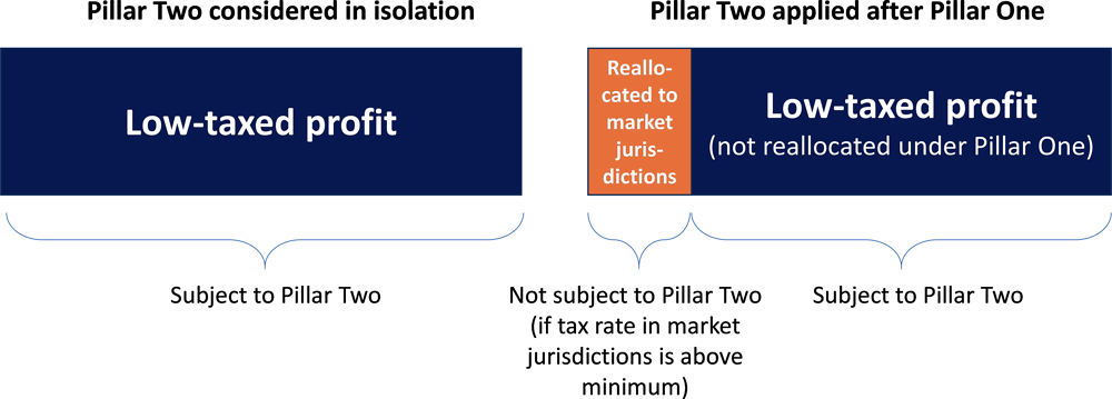
Source: OECD Secretariat.
224. In this example, computing the revenue gains from Pillar One and Pillar Two independently of each other would overstate the overall gains compared to computing the joint effect of both pillars in a way that takes into account the interaction between them. It is possible to consider an opposite example, where the reallocation taking place under Pillar One would increase the amount of low-taxed profits and therefore increase the revenue gains from Pillar Two. This would be the case for example if an MNE group had most of its profit located in higher-tax jurisdictions and most of its sales in low-tax jurisdictions. However, in practice, MNE profit tends to be more concentrated in low-tax jurisdictions than MNE final sales, which is why the reallocation taking place under Pillar One is expected to reduce the global amount of low-taxed profit. Therefore, taking into account the interaction with Pillar One is expected to reduce the estimated revenue gains from Pillar Two.
3.5.2. Methodology on the interaction between both pillars
225. To take the interaction between both pillars into account, Scenario 2 applies Pillar Two in exactly the same way and with the same assumptions as in Scenario 1, but after adjusting the location of profit for the reallocation induced by Pillar One. In practice, this is done by computing an adjusted profit matrix post Pillar One reallocation. Each matrix cell (corresponding to the profit in jurisdiction i of MNE groups with an ultimate parent in jurisdiction j) is adjusted in the following way:
226. The amount of profit received and relieved under Pillar One in each matrix cell is based on the Pillar One estimates described in Chapter 2.24 In theory, this adjustment can be done for any combination of Pillar One parameter and design options. For simplicity, only one illustrative set of Pillar One design and parameter assumptions among those explored in Chapter 2 is considered in this chapter (i.e. residual profit threshold percentage of 10%, reallocation percentage of 20% and global revenue threshold of EUR 750 million).
3.5.3. Results on Scenario 2
227. The resulting profit matrix, adjusted for Pillar One reallocation is presented in Table 3.7. Compared to the original profit matrix (Table 3.1), the total in each column is the same (by construction), but there has been some reallocation across rows, away from investment hubs and into other jurisdiction groups. The scale of this reallocation is limited, which implies that the global amount of low-taxed profit and the estimated revenue gains from Pillar Two are reduced only slightly by taking into account the interaction with Pillar One (Table 3.8). To the extent that the interaction with Pillar One has only a modest effect on Pillar Two results, considering different assumptions regarding Pillar One would likely affect the Pillar Two estimates only at the margin.
228. Scenario 3 is based on the assumption that MNE profit shifting intensity would be reduced by the introduction of Pillar Two. This is because Pillar Two would reduce tax rate differentials between jurisdictions, which are a primary driver of profit shifting. The effect of this reduced profit shifting intensity on tax revenues is estimated based on the assumption that profit shifting generally depends on tax rate differentials, and by comparing tax rate differentials before and after Pillar Two implementation. An adjusted profit matrix incorporating the reduced profit shifting intensity is derived from this comparison, as further described below.
229. Based on this adjusted profit matrix, revenue gains from Pillar Two in Scenario 3 are computed as the sum of two components: (i) a revenue effect of the reduction in profit shifting intensity, reflecting that profits that are no longer shifted are now taxed in the jurisdiction where they were generated, rather than in the jurisdiction where they used to be shifted, and (ii) revenues collected via the IIR and UTPR on remaining low-taxed profits, including profits that are still shifted to low-tax jurisdictions. This second component is expected to be smaller than the amount of revenues collected in Scenario 2, since the reduction in profit shifting should reduce the global amount of low-taxed profit. However, the sum of the two components is expected to be greater than the overall revenue gains in Scenario 2, since some profit that is no longer shifted to low-tax jurisdictions may ultimately be taxed at a higher rate than the minimum rate in the jurisdictions where it has been generated.
3.6.1. Assessing current profit shifting patterns
230. To evaluate the effect of Pillar Two introduction on MNE profit shifting patterns, the first step is to assess current profit shifting patterns. For consistency with the methodology applied to quantify the revenue effects of Pillar Two in this chapter, profit shifting needs to be assessed on a “trilateral” basis, i.e. for each combination of (i) jurisdiction where profit was located before shifting (“profit origin”), (ii) jurisdiction where profit has been shifted (“profit destination”), and (iii) jurisdiction of ultimate parent of the profit shifting entity (“ultimate parent”).25 This third jurisdiction may or may not be the same as the “profit origin” jurisdiction. This level of granularity is necessary to create an adjusted profit matrix taking into account the effect of Pillar Two on profit shifting intensity, so that Pillar Two can then be applied to this adjusted profit matrix (with assumptions consistent with those used in Scenarios 1 and 2). This requires going beyond most studies on profit shifting, which often focus on measuring an average profit shifting semi-elasticity across a range of destination jurisdictions – for recent reviews of these studies, see for example Bradbury et al. (2018[11]) and Beer et al. (2019[12]).
Profit shifting: Overview of the approach
231. To obtain this “trilateral” profit shifting intensity, the approach in this chapter is based on the following steps, which are further detailed in the following sections and presented in a stylised way in Figure 3.7:
(i) Identifying “profit destination” jurisdictions, i.e. jurisdictions where profit may have been shifted to, based on foreign direct investment (FDI) and ETR data;
(ii) Computing the amount of deemed shifted profit in these jurisdictions, assuming that profit up to a certain “normal” profitability rate may not have been shifted, but may instead reflect real economic activity in these jurisdictions. The share of shifted profit is measured on a “bilateral” basis, i.e. for each pair of “profit destination”-“ultimate parent” jurisdictions;
(iii) Identifying where the shifted profit originates from. For each “profit destination”-“ultimate parent” pair of jurisdictions, shifted profits need to be reattributed to “profit origin” jurisdictions. This is done based on tax rate differentials vis-à-vis the “profit destination” jurisdiction (assuming that a higher tax rate differential leads to more profit shifting, all else equal) and on the geographic distribution of economic activity of MNEs from the “ultimate parent” jurisdiction considered (with the idea that profit is more likely to originate from jurisdictions where these MNEs have more economic activity).
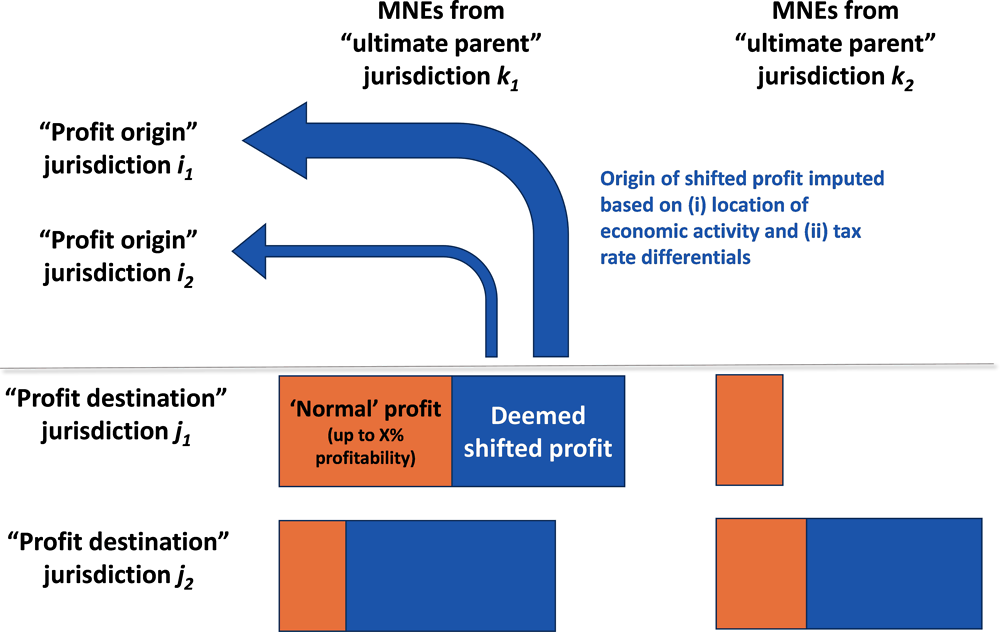
Note: In this stylised example, only two “ultimate parent” jurisdictions, two “profit origin” jurisdictions and two “profit destination” jurisdictions are represented. In reality, all jurisdictions in the profit matrix (more than 200 jurisdictions) are considered as “ultimate parent” jurisdictions, and all jurisdictions in the profit matrix are either “profit origin” or “profit destination”, based on the criteria described in the next section (using FDI and ETR data). For each pair of “ultimate parent”-“profit destination” jurisdictions, profit up to a certain profitability rate is deemed ‘normal’ (orange bars), and the rest, if any, is deemed shifted (blue bars). In this example, some profit in the k1-j1, k1-j2 and k2-j2 pairs is deemed shifted, but not in the k2-j1 pair. Deemed shifted profit is assumed to originate from “profit origin” jurisdictions in a way that depends on the location of the MNEs’ economic activity and tax rate differentials, as further described below. This is materialised by the blue arrows in the figure – in this example, profit in the k1-j1 pair is found to come predominantly from jurisdiction i1 (thick arrow) and to a lesser extent from jurisdiction i2 (thin arrow). The corresponding arrows identifying the origin of profit deemed shifted in jurisdiction pairs k1-j2 and k2-j2 are not represented to avoid overburdening the figure.
Source: OECD Secretariat.
232. This approach to measuring profit shifting is new, although it shares some common features with Tørsløv et al. (2018[5]), Cobham et al. (2019[13]) and Clausing (2020[8]). The approach is enabled by the level of detail offered by the profit matrix and the underlying data sources, including anonymised and aggregated CbCR data, which give a detailed account of the amount of profit located across low-tax jurisdictions for each ultimate parent jurisdiction. To benchmark the results against the vast existing literature on profit shifting, an average aggregate profit shifting semi-elasticity is computed based on the results and compared with existing estimates of this semi-elasticity.
Profit shifting: Identifying “profit destination” jurisdictions
233. Potential “profit destination” jurisdictions are assumed to be those meeting at the same time both of the following two criteria:
Having an inward FDI-to-GDP ratio above 100%, as computed based on hard or extrapolated FDI data (see Annex 5.C of Chapter 5 on the FDI extrapolation methodology);26
Having an average ETR on MNE profit below 17.5%, based on the median of the three data sources considered in Section 3.4.2 above. This rate of 17.5% is not meant to represent an ETR ceiling above which profit shifting would not occur. Indeed, there may be profit shifting taking place between jurisdictions with higher rates than 17.5%. Instead, this rate is the highest rate in the range of potential minimum rates illustratively considered in this chapter. Since the incentive to shift profit into jurisdictions with an average ETR above the minimum rate would not be directly affected by Pillar Two as modelled in this chapter,27 the focus in this chapter is exclusively on profit shifting into jurisdictions with an average ETR below the minimum rate. For example, when the minimum rate is assumed to be 12.5%, only profit shifting to jurisdictions with an average ETR below 12.5% is assumed to be modified by Pillar Two.28
234. Based on these criteria, 39 jurisdictions are identified as potential “profit destinations”. However, not all of them host deemed shifted profit, as this also depends on the profitability rate of MNEs in the jurisdiction (see next section). Overall, the list of jurisdictions with substantial amounts of deemed shifted profit overlaps widely with other lists in the literature, such as Tørsløv et al. (2018[5]), which often relate to the early list developed by Hines and Rice (1994[14]).
Profit shifting: Separating deemed shifted profit from “normal” profit
235. In these potential “profit destination” jurisdictions, only a share of reported profits are deemed shifted. This is because MNEs can have local economic activity in these jurisdictions, which generate local (non-shifted) profits. To account for this, only profit above a certain “normal” profitability rate is deemed shifted. This normal profitability rate is set at 7.9% (on the ratio of pre-tax profit to turnover) in the baseline estimates, which corresponds to the average global profitability of MNEs observed in the ORBIS sample.29 Robustness checks have been performed with other rates, including 5% and 10%. They give results that are qualitatively similar to the baseline (Table 3.9).
236. Based on data in the profit matrix and data on ETRs from Section 3.4.2, estimates of shifted profit are derived for each “profit destination”-“ultimate parent” jurisdiction pair. At the aggregate level, the amount of deemed shifted profit is estimated to be about USD 650-850 billion, or about 10-14% of global MNE profit (Table 3.9).30 This is broadly consistent with the estimates of USD 741 billion and USD 667 billion obtained by Tørsløv et al. (2019[15]; 2019[16]), which are updates, for 2017 and 2016 respectively, of their earlier USD 616 billion figure for 2015 (Tørsløv, Wier and Zucman, 2018[5]). The share of deemed shifted profit in total profit tends to be higher among zero tax jurisdictions (88-94%) than in other “profit destination” jurisdictions (55-74%), which is in line with the intuition that there is less economic substance (and therefore a greater share of shifted profits) in zero-tax jurisdictions than in other “profit destination” jurisdictions.
Profit shifting: Identifying “profit origin”
237. Once shifted profit has been identified, further assumptions are required to identify where profit originates from, i.e. the jurisdiction where it was generated before being shifted. This is done at the level of each “profit destination”-“ultimate parent” pair, using the following formula:
238. In this formula, is the amount of profit shifted from jurisdiction i to jurisdiction j by MNEs with an ultimate parent in jurisdiction k. The intuition is that this profit is proportional to the economic activity in i of MNEs with an ultimate parent in k. For example, an MNE with very little economic activity in a jurisdiction is unlikely to have profit shifted away from this jurisdiction, whatever the tax rate differential with this jurisdiction. This economic activity is proxied by the turnover in i of MNEs with an ultimate parent in jurisdiction k (denoted ) sourced from the turnover matrix.31 Results are broadly robust to using tangible assets or payroll instead of turnover (Annex 3.C).
239. The amount of shifted profit is also assumed to be a function of the tax rate differential between jurisdictions i and j: . The tax rates considered are the statutory CIT rates in “profit origin” jurisdictions, in line with most of the profit shifting literature that focuses on statutory rates, and the ETRs in “profit destination” jurisdictions (with the same data sources as in the rest of this chapter), as ETRs sometimes differ considerably from statutory rates in these jurisdictions. Several shapes of the relationship between profit shifting intensity and tax rate differentials (i.e. of the function ) are explored in this chapter, as further discussed below.
240. Finally, the amount of profit shifted depends on an array of scaling factors, which are specific to each “profit destination”-“ultimate parent” pair of jurisdictions. These scaling factors capture that certain “profit destination” jurisdictions are more attractive to MNEs of a given “ultimate parent” jurisdiction – owing to, for example, geographic proximity or the legal environment – and that tax rate differentials alone do not predict where shifted profits are located. Instead of being taken from the literature, or set at arbitrary levels, these factors are set at the unique level that is consistent with the amount of profit that is deemed shifted in each “profit destination”-“ultimate parent” pair of jurisdictions, as computed in the previous section. Formally, these factors are computed based on the following formula:
241. This way of defining the factors ensures the consistency of the approach, in the sense that the total profit attributed across “profit origin” jurisdictions – for a given “profit destination”-“ultimate parent” pair of jurisdictions – corresponds exactly to the total profit deemed shifted in that pair of jurisdictions. Ultimately, the average of these factors can be compared to estimates of the profit sensitivity to tax rate differentials from the literature, as further discussed below.
242. A central question is the shape of the function, i.e. the relationship between profit shifting and tax rate differentials. This is important for the modelling of profit shifting in this section, but also because this assumption defines the way in which reduced tax rate differentials under Pillar Two will affect profit shifting intensity. The academic literature offers limited insights in this area. Most studies assume a linear relationship between profit shifting and statutory tax rate differentials and find evidence that this relationship is significant, but do not test empirically for other potential shapes (see for example Bradbury et al. (2018[11]) and Beer et al. (2019[12]) for recent reviews). Such a linear relationship is consistent with the theoretical framework of Huizinga and Laeven (2008[17]), which is based on the underlying assumption that the cost of profit shifting is quadratic. With this assumption, an “interior” solution to the MNE’s profit maximisation problem implies that profits are shifted in proportion to tax rate differentials.
243. However, some recent studies suggest that the position is more complex in reality. In particular, Bilicka (2019[18]) and Johannesen et al. (2019[19]) show that many MNE entities report zero profit in higher-tax jurisdictions. This would suggest that these MNEs are able to shift all their profit from these jurisdictions, in which case the solution to the MNE’s profit maximisation problem is not always “interior” and the relationship between profit shifting and tax rate differentials is no longer linear. Also, Dowd et al. (2017[20]) find a non-linear relationship according to which US MNEs shift more profits to jurisdictions with very low tax rates than a linear elasticity would imply.32 However, the question considered in that paper is somewhat different from the one considered in this chapter. Indeed, Dowd et al. (2017[20]) focus on the choice of potential “profit destination” jurisdictions for a given “ultimate parent” jurisdiction (in which case, the fact that MNEs shift as much profit as possible to jurisdictions with the lowest ETRs seems intuitive), while this chapter aims to identify “profit origin” jurisdictions for given “ultimate parent” and “profit destination” jurisdictions.
244. Another insight from the literature is that, all else equal, profit shifting tends to be more intense in lower income jurisdictions than in higher income ones. For example, Fuest et al. (2011[21]), based on German micro-data, find that profit shifting via intra-company loans is approximately twice as intense among the developing countries in their sample compared to other jurisdictions, which they suggest may be due to the limited capacity of these jurisdictions to enforce anti-tax avoidance policies. Johannesen et al. (2019[19]) find that a 10 percentage point decrease in foreign affiliates’ tax rates increases the likelihood that an MNE reports zero profits by 3 percentage points in low/middle income countries, but only by 1.7 percentage points in high income countries, based on firm-level data from ORBIS. Finally, Cobham and Janský (2018[22]) relying on macro data, find that “the intensity of losses is substantially greater in low‐income and lower middle‐income jurisdictions; and in sub‐Saharan Africa, Latin America and the Caribbean and in South Asia compared with other regions.”
245. Against this background, the baseline assumption in this chapter is that profit shifting is generally proportional to tax rate differentials, but more intense in lower income jurisdictions than in higher income ones. Formally, the function is assumed to be defined as follows: if is positive, and zero otherwise. The coefficient is equal to 1 in high income jurisdictions, 1.5 in middle income ones and 2 in low income jurisdictions (based on the World Bank classification of jurisdictions by income groups). This shape of the relationship between profit shifting and tax rate differentials is presented in Figure 3.8. As discussed above, the absolute amounts of shifted profit attributed to each “profit origin” jurisdiction will depend on the assumptions presented in this figure, but also on the factors that capture the amount of deemed shifted profit in each “profit destination” jurisdiction (and for each “ultimate parent” jurisdiction).
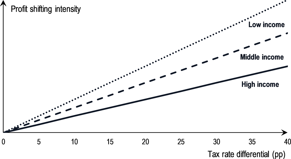
Note: Under the assumptions presented in this figure, the intensity of profit shifting to a jurisdiction is assumed to be proportional to the tax rate differential vis-à-vis this jurisdiction. Profit shifting intensity is assumed to be 1.5 times (resp. 2 times) higher for profit shifted from middle income (resp. low income) jurisdictions compared to high income jurisdictions. The amount of shifted profit (i.e. scale of the Y-axis) will depend on the factors defined above, which capture the amount of deemed shifted profit in each “profit destination” jurisdiction (and for each “ultimate parent” jurisdiction ).
Source: OECD Secretariat.
Profit shifting: Alternative shapes of the relationship between profit shifting and tax rate differentials
246. To account for potential non-linearities in the shape of the relationship between profit shifting and tax rate differentials, alternative shapes are considered as robustness checks. These shapes are used for the purpose of creating uncertainty ranges around the estimates.
247. Two alternative shapes are considered. The first one is based on the idea that lower income jurisdictions may suffer from profit shifting for tax but also non-tax-related reasons. For example, investors may shift profits away from these jurisdictions due to fears of political instability and/or to circumvent capital controls (this may also be the case in high income jurisdictions, but it seems likely to be less frequent than in lower income jurisdictions). As a result, profit shifting may exist in these jurisdictions even for relatively low tax rate differentials and the subsequent slope of the relationship between profit shifting and tax rate differentials may be less steep than envisaged in the baseline (Figure 3.9, Panel A). This shape also takes into account the assumption that under relatively small tax rate differentials (i.e. less than 5 percentage points), MNEs may generally consider that the costs of profit shifting would exceed the gains (in terms of tax savings). This is why in Figure 3.9 (Panel A) profit shifting intensity does not increase with the tax rate differential as long as this differential remains below 5 percentage points.
248. The second alternative shape takes the same starting point, but also assumes that the slope of the relationship becomes less steep – across all income groups – above a certain level. The idea is that above a certain tax rate differential, MNEs’ profit shifting incentives are high anyway and, as a result, these incentives would not be greatly affected by marginal changes in tax rate differentials (Figure 3.9, Panel B).
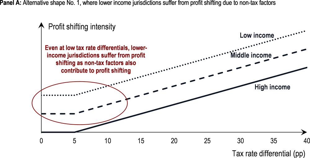
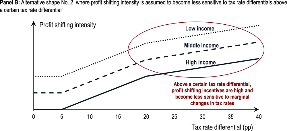
Note: In Panel A, profit shifting intensity is assumed to be higher among lower income jurisdictions than higher income jurisdictions, as in the baseline (Figure 3.8). However, profit shifting in lower income jurisdictions is assumed to be partly driven by non-tax factors, which implies that lower income jurisdictions face profit shifting even under low (or even zero) tax rate differentials. In turn, reducing tax rate differentials in lower income jurisdictions tends to reduce profit shifting less than in the baseline scenario. In Panel B, this assumption is kept, and, in addition, profit shifting intensity is assumed to become less sensitive to tax rate differentials above a certain tax rate differential. This could reflect that for relatively high tax rate differentials, the incentive to shift profit is high anyway, and therefore less influenced by the exact level of the rate differential. In both panels, the amount of shifted profit (i.e. scale of the Y-axis) will depend on the factors defined above, which capture the amount of deemed shifted profit in each “profit destination” jurisdiction (and for each “ultimate parent” jurisdiction ).
Source: OECD Secretariat.
Profit shifting: Comparing the aggregate semi-elasticity with the literature
249. The estimates obtained with the methodology described in the previous sections can be compared with the existing literature by computing an average aggregate semi-elasticity of profit to tax rate differentials. In practice, this means computing a weighted average of the coefficients. In the baseline case described above, this aggregate profit shifting elasticity is estimated to be about 1.2.33 This estimate is close to the semi-elasticity of 1 that was found in a recent meta-analysis by Beer et al. (2019[12]). An earlier meta-study found a semi-elasticity of 0.8 (Heckemeyer and Overesch, 2017[23]) The semi-elasticity found in earlier OECD estimates produced in the context of the BEPS Action 11 report was also about 1 (OECD, 2015[24]; Johansson et al., 2017[25]). Overall, this suggests that the methodology to assess profit shifting in this chapter, while based on an approach and on data sources different from most earlier studies, is broadly consistent with these studies in terms of overall results, as suggested as well by the results in Table 3.9.
3.6.2. Impact of Pillar Two on tax rate differentials and profit shifting
250. Pillar Two is expected to reduce tax rate differentials between jurisdictions. More precisely, it is expected to reduce the tax rate differential vis-à-vis jurisdictions where the ETR is currently below the minimum rate, by increasing this ETR up to the level of the minimum rate. In a scenario where governments in these jurisdictions do not react, as in Scenario 3, this minimum rate would be paid in another jurisdiction (e.g. the jurisdiction of the ultimate parent in the case of the IIR). If some of the jurisdictions with an ETR below the minimum rate increase their ETR up to the minimum tax rate, as envisaged in Scenario 4, then the tax would be paid in these jurisdictions.
251. In both of these cases, the incentives of MNEs to shift profit to low-tax jurisdictions would be reduced compared to a scenario without Pillar Two. It is also useful to note that these incentives would be the same regardless of whether governments in low-tax jurisdictions increase their ETR or not, since the MNE would face the same amount of tax on its shifted profit (the only difference being where this tax is paid). This is why the order in which the MNE and government reactions are considered in this chapter has relatively little impact on the final outcome, as mentioned earlier.34
252. Profit shifting intensity is assumed to be substantially reduced by the decline in tax rate differentials induced by Pillar Two. However, profit shifting is not expected to be completely eliminated by Pillar Two, since some tax rate differentials would persist between the minimum rate and the (higher) rate that applies in the jurisdictions with an ETR above the minimum rate (see stylised example in Figure 3.10). In practice, the decision of an MNE group to continue or not with a certain profit shifting scheme will depend on the tax rate differential after the implementation of Pillar Two and the costs of the profit shifting scheme (e.g. financial and advisory costs associated with setting up the scheme, reputational costs). In some cases, the MNE group may continue with the scheme, while in others it may find that the costs will outweigh the benefits after Pillar Two is introduced. It is difficult to assess how frequent the decision to reduce or even stop profit shifting will be, since the costs of profit shifting are not known with precision and will vary across MNE groups and jurisdictions.
253. In addition, MNE decisions may be more complex than a simple choice between continuing or stopping a profit shifting scheme, as a possible alternative may be to create a different scheme to shift profit to another jurisdiction (e.g. a jurisdiction with a higher ETR but to which the costs of shifting profit are lower) including potentially through changes in corporate structure.35 These complex reactions will depend on the particular circumstances and choices of each MNE group, and modelling them goes beyond the ambition of this chapter. If MNE reactions depart significantly from the stylised modelling assumptions used in this chapter, which are described below, this could significantly affect the estimated Pillar Two revenue effects, especially at the level of individual jurisdictions. At the global level, or for broad jurisdiction groups, the effect of different profit shifting reactions could partly cancel each other (e.g. if one jurisdiction in the group receives more profit, another jurisdiction in the group may receive less).
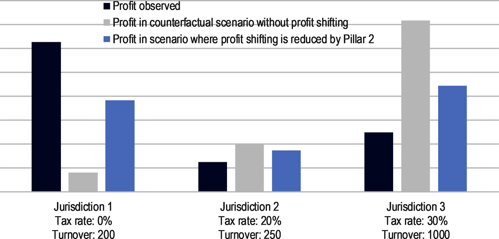
Note: This stylised example, based on fictitious numbers, illustrates how Pillar Two may reduce profit shifting but not eliminate it. In the current situation, most of the profit of the MNE group considered is located in Jurisdiction 1, which has a 0% tax rate. Most of this profit is deemed shifted, which is why little profit remains in Jurisdiction 1 in the counterfactual scenario without profit shifting. This profit is reallocated to Jurisdictions 2 and 3 based on the modelling on profit shifting described above. In the scenario where profit shifting is reduced by Pillar Two (assuming illustratively a 12.5% minimum tax rate), a greater share of profit remains in Jurisdiction 1 as the tax rate differential vis-à-vis Jurisdictions 2 and 3 is reduced but not eliminated.
Source: OECD Secretariat
254. Against this background, the stylised baseline assumption in this chapter is that profit shifting would be reduced proportionally to the reduction in tax rate differential induced by Pillar Two. For example, if Pillar Two reduces the tax rate differential between two jurisdictions by a third, profit shifting between these two jurisdictions is assumed to be reduced by a third. This assumption is consistent with the baseline modelling of profit shifting above.
255. However, this assumption overlooks the fact that (i) some profit shifting in lower income jurisdictions is related to non-tax factors and may persist after the introduction of Pillar Two, and (ii) that for high tax rate differentials, a marginal change in the tax rate differential may not lead to much of a change in the profit shifting intensity, since the profit shifting incentive is high anyway (put differently, the gain from profit shifting outweighs the costs in this case by such a large amount, that a marginal reduction in this gain would not change the choice of the MNE group to engage in profit shifting). These considerations are taken into account in the robustness check scenarios based on the two alternative shapes of the relationship between profit shifting intensity and tax rate differentials (Figure 3.9). In particular, with the second shape, profit shifting incentives become less sensitive to tax rate differentials when these differentials are relatively high. These two robustness check scenarios are used to build the uncertainty ranges around the estimates.
256. Based on the assumptions described above, an adjusted profit matrix taking into account the reduced profit shifting intensity is presented in Table 3.10 for an illustrative minimum tax rate of 12.5%. This is done for the baseline shape of the relationship between profit shifting intensity and tax rate differentials (Panel A) and for the two alternative shapes from Figure 3.9 (Panels B and C). Compared to Table 3.7, the total amount of profit in each column is the same (by construction), but the location of profit has shifted across matrix rows. Broadly speaking, profit has been reallocated away from investment hubs and into the other jurisdiction groups. The amount of profit in investment hubs is reduced by about 9-10% compared to Table 3.7 (depending on the panel considered) and the amount of profit in other jurisdiction groups is increased by 1-8% depending on the group and the panel considered. In particular, middle and low income jurisdictions tend to regain less profit under the alternative shapes of the relationship between profit shifting intensity and tax rate differentials (Panels B and C) than under the baseline (Panel A), which is consistent with the assumptions underlying these alternative shapes and discussed in the previous section.
3.6.3. Implications of a formulaic substance-based carve-out on profit shifting behaviour
257. The estimates in the previous section are based on a scenario where Pillar Two would not include a formulaic substance-based carve-out. This section discusses how the inclusion of a potential formulaic substance-based carve-out could modify the effect of Pillar Two on MNE profit shifting incentives.
258. A formulaic substance-based carve-out could have two main effects regarding MNE profit shifting behaviour. First, a carve-out might in theory reduce the effect of Pillar Two on profit shifting in specific situations where an MNE group would shift profit to a jurisdiction where it already has a substantial amount of tangible assets and/or payroll. In practice, this is not likely to be the case very often, as profit is frequently (and more likely) shifted to jurisdictions where MNE groups have minimal levels of substantive activity (see Table 3.5 for example). For example, assuming that, after the introduction of Pillar Two, (i) incentives to shift profit are not modified by Pillar Two as long as the shifted profit is ultimately carved out under Pillar Two, and that (ii) Pillar Two has the same effect on the shifting of ‘non-carved-out profit’ as in the no-carve-out case,36 then the effect of Pillar Two on the global amount of shifted profit would be reduced by less than 1% compared to a situation where Pillar Two is applied without carve-out.37
259. Second, the existence of a formulaic substance-based carve-out could encourage MNE groups to relocate tangible assets or employees to low-tax jurisdictions where they already shift profit (or could shift profit in the future) in order to benefit from the carve-out. This effect is difficult to model as it depends on the cost of relocating tangible assets or employees across jurisdictions, which is specific to each MNE group and each jurisdiction. In practice, tangible assets and employees are generally less mobile than intangible assets. Under the carve-out percentages considered in this chapter, it seems unlikely that a substantial amount of relocation would take place.38 Still, a formulaic substance-based carve-out may trigger attempts by tax planning MNEs to reclassify the location of tangible assets or employees for tax purposes without changing significantly their actual physical location, or to resort to other schemes to try to benefit from the carve-out without actually relocating tangible assets or employees. Reflecting this, it is important that the design of the carve-out is ‘abuse-proof’, in the sense that it opens carve-out rights only when justified by the actual location of tangible assets and/or employees.
260. Against this background, the estimates in this chapter assume that the effect of Pillar Two on profit shifting intensity are the same in the scenarios with a formulaic substance-based carve-out as in the no-carve-out scenario.
3.6.4. Global Pillar Two revenue gains under Scenario 3
261. Revenue gains from Pillar Two under Scenario 3 are computed based on the assumptions described in the previous sections and presented in Table 3.11. For simplicity, only point estimates are presented, and ranges reflecting uncertainty relative to pockets of low-taxed profits are not included in this table (these ranges are included in the summary tables presented in Section 3.9). The revenue gains consist of two components:
Effect of the reduced profit shifting intensity: Profit that is no longer shifted is assumed to be taxed at the statutory CIT rate in the “profit origin” jurisdictions where it was generated. This assumption is consistent with the literature on profit shifting, which generally assumes that the marginal tax rate that would otherwise be applied to shifted profit is the statutory rate.39 In contrast, “profit destination” jurisdictions would receive less shifted profit, leading them to lose tax revenues. For these jurisdictions, it is assumed that the shifted profit was taxed at the average ETR on MNE income, reflecting that some of these jurisdictions tax MNE profit at a rate that is well below the statutory rate.40 Overall, at the global level, the net result is a tax revenue gain, since the tax rate applied in “profit origin” jurisdictions tends is higher than in “profit destination” ones.
Revenues collected via the minimum tax: Even if MNE profit shifting intensity is reduced, some profit would remain located in jurisdictions where the ETR is below the minimum rate. Profit in these jurisdictions would be subject to the IIR and UTPR (except regarding US MNEs, where they would be subject to GILTI), which are modelled with the same assumptions as in Scenarios 1 and 2. The interaction with Pillar One is taken into account in the same way as in Scenario 2, based on the profit matrix adjusted for the new profit shifting patterns.
262. To reflect the uncertainties around the estimates, results in the final section of this chapter are presented as ranges. In the case of the effect of reduced profit shifting, the range is defined in the following way: for each jurisdiction, the bottom (top) point of the range is the minimum (maximum) value across the results obtained with the three shapes of the relationship between profit shifting intensity and tax rate differentials considered in this chapter (baseline and alternative shapes No. 1 and No. 2, as described in Figure 3.8 and Figure 3.9).
263. In Scenario 4, it is assumed that certain jurisdictions would change some of their tax rules and/or rates to increase their jurisdiction’s ETR on profit that is currently taxed below the minimum rate. The rationale for this reaction is that an ETR increase (up to a rate below or equal to the minimum rate) would not necessarily change the overall amount of tax paid by MNEs, but it would allow the jurisdictions increasing their ETR to capture a greater share of global tax revenues.
264. In practice, whether such an ETR increase would change the overall amount of tax paid by MNEs or not would depend on the design of Pillar Two and of the MNE considered. In particular, assuming that Pillar Two includes a formulaic substance-based carve-out, an ETR increase could increase the overall amount of tax paid by some MNEs, as they would ‘lose the benefit’ of the carve-out in the jurisdictions increasing their ETR (i.e. they would have to pay the minimum tax rate on all their profit, including the profit that was carved-out under Pillar Two).41,42 In the case of US MNEs, under the illustrative assumption that GILTI would coexist with Pillar Two, an ETR increase by a low-tax jurisdiction would also lead to a higher overall amount of tax paid.43
265. The uncertainty over whether a local ETR increase would increase the global amount of tax paid by MNEs or not makes it difficult to assess with certainty which jurisdictions would decide to increase their ETR in reaction to Pillar Two. Other considerations that are discussed in the next section (e.g. administrative costs of creating a CIT system in a jurisdiction where there is none, possible knock-on effects on taxes paid by non-MNE firms) also add to this uncertainty. Reflecting this, the assumptions presented in the next section should be seen as nothing more than stylised and illustrative assumptions.
3.7.1. Assumptions on government reactions
266. The modelling of Scenario 4 in this chapter is based on the following assumptions on government reactions. These assumptions, which are summarised in Table 3.12, are consistent with those made on Pillar Two implementation in Section 3.4.5 above. They do not depend on the assumption made on a potential formulaic substance-based carve-out, even though, as discussed above, such a carve-out would tend to reduce the incentives for low-tax jurisdictions to increase their ETR.
Group 1: Jurisdictions with an average ETR above the minimum rate. No reaction is modelled. This is because, as discussed above, the potential policy reaction of jurisdictions with an ETR above the minimum rate is a priori ambiguous.44
Group 2: Jurisdictions with a zero corporate tax rate. For the purposes of the modelling in this chapter, jurisdictions in this group are not assumed to increase their ETR. The reason is that these jurisdictions generally do not have a CIT system. Introducing a corporate tax system from scratch would generate significant administrative costs, could lead these jurisdictions to be seen as less attractive investment destinations, and could also have spillovers on other sectors of their economies since non-MNE firms would possibly have to be subject to the newly-introduced CIT as well. Assuming that Pillar Two includes a formulaic substance-based carve-out, an additional argument is that an ETR increase would no longer be neutral for the overall amount of tax paid by MNEs, as discussed above. Under the assumption that GILTI would coexist with Pillar Two, the ETR increase would not be neutral for US MNEs either.
Group 3: Jurisdictions with an average ETR below the minimum rate, but greater than zero. Jurisdictions in this group have a CIT system, so it is easier for them to increase their ETR than for jurisdictions in Group 2. Still, it seems plausible that not all of them will increase their ETR, including for the reasons discussed above. In addition, the ETRs faced by MNEs may not be homogeneous, as they reflect the application of different tax provisions (e.g. different kinds of tax deductions and preferential regimes), in which case it may not be straightforward to bring the ETR of all MNE entities up to the level of the minimum rate. Against this background:
The assumption in this chapter is that half of jurisdictions in Group 3 would increase their ETR on the profit of MNEs up to the level of the minimum rate under Pillar Two, while the other half would not. This is consistent with the assumptions on IIR and UTPR implementation, described in Section 3.4.5, where half of jurisdictions in this group are assumed to implement an IIR and a UTPR. Potential revenue gains related to an increase in the ETR of non-MNE entities are not taken into account in this chapter.
In practice, and as above, identifying the jurisdictions in Group 3 that would increase their ETR is not straightforward and a similar methodology as used for IIR and UTPR implementation in Scenario 1 is applied. Instead of arbitrarily selecting half of the jurisdictions in the group, a simplifying assumption is made that all jurisdictions in this group increase their ETR to close half of the gap vis-à-vis the minimum rate. Again, this does not aim to be realistic in itself, but rather to be a reasonable proxy for a situation where half of the jurisdictions in this group would increase their ETR to the level of the minimum rate and the other half would not change their ETR. For the purpose of creating uncertainty ranges around the estimates, it is assumed that between one-third and two-thirds of jurisdictions in this group would increase their ETR to the level of the minimum rate (instead of one-half in the baseline).
3.7.2. Scenario 4 methodology and results
267. The methodology to compute revenue gains from Scenario 4 is relatively straightforward, since the location of profit is the same as in Scenario 3 (Table 3.10). The main difference with Scenario 3 is the distribution of revenue gains across jurisdictions, as jurisdictions increasing their ETR capture a greater share of global revenue gains. In practice, jurisdiction-specific gains are computed consistently with Scenarios 1-3 above, with the additional assumption that profit in a jurisdiction increasing its ETR is taxed by this jurisdiction, instead of being subject to the IIRs and UTPRs of other jurisdictions (Figure 3.11).
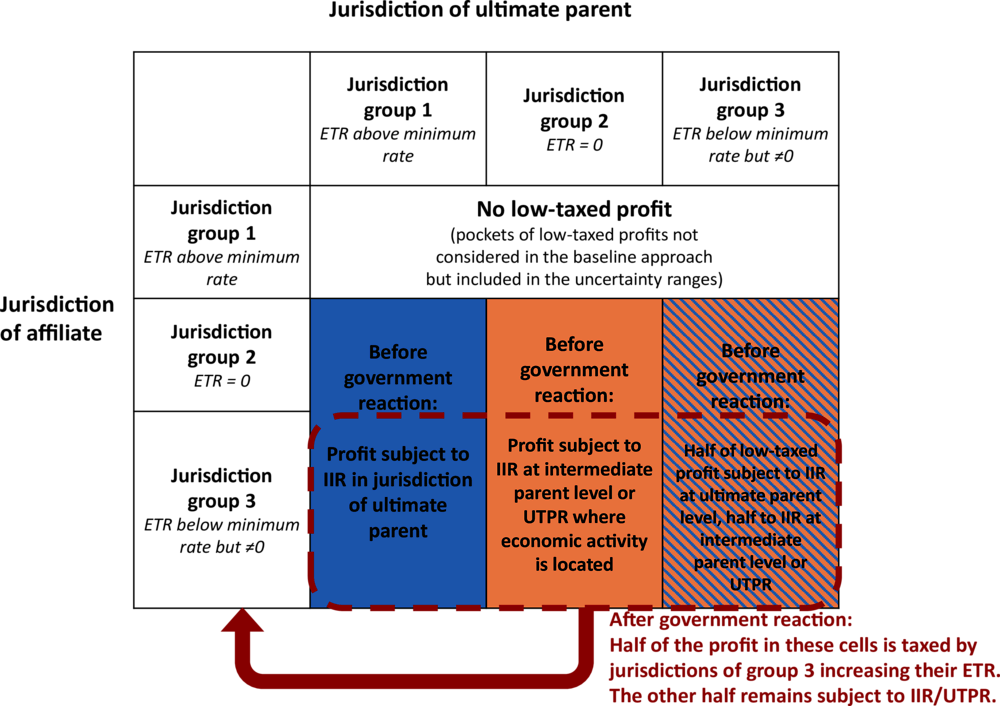
Note: This stylised figure illustrates how the reaction of governments is taken into account in Scenario 4. For the sake of simplicity, this figure focuses on a scenario without formulaic substance-based carve-out. Compared to the similar illustration for Scenarios 1-3 (see Figure 3.5), half of the profit located in countries from group 3 is taxed by these countries as they increase their ETR. The other half of this profit remains subject to IIR and UTPR as in Scenarios 1-3.
Source: OECD Secretariat.
268. Global revenue gains in Scenario 4 are presented in Table 3.13. For simplicity, only point estimates are presented, and ranges reflecting uncertainty relative to pockets of low-taxed profits are not included in this table (these ranges are included in the summary tables presented in Section 3.9). Also for simplicity, results in Table 3.13 only focus on the baseline shape of the relationship between profit shifting intensity and tax rate differentials. Results for the two alternative shapes discussed above are presented in Annex 3.A.
269. As discussed above, while no decision has been taken by the Inclusive Framework yet, it is illustratively assumed in this chapter that GILTI would coexist with Pillar Two. This is assumed to imply that the United States would collect revenues from GILTI, instead of the IIR, on the low-taxed foreign profit of US MNEs.
270. GILTI shares some common characteristics with GloBE, in the sense that it results in a minimum level of taxation on the foreign profit of US MNEs, but also differs from GloBE in a number of ways. An important difference is the level of blending, as GILTI involves largely, but not completely, global blending of foreign profit, while GloBE (under the illustrative assumptions in this chapter) would entail jurisdictional blending. Other differences (also depending on the final design of GloBE) may notably include the existence of a global revenue threshold, the exact definition of the tax base, the inclusion of loss carry-forward and tax-credit carry-forward provisions, the definition of covered taxes as well as the existence and design of potential carve-outs (see Pillar Two Blueprint report). The GILTI tax rate ranges between 10.5% and 13.125% depending on the amount of foreign taxes paid.45 These rates are scheduled to increase to 13.125%-16.406% in 2026. GILTI applies to profit in excess of 10% of the carrying cost of tangible assets used in the production of GILTI income reduced by certain interest expense (based on so-called “qualified business asset investment”).
271. It goes beyond the ambition of this chapter to model with precision the revenue gains from GILTI, due notably to the many potential rule differences with GloBE. Ex ante estimates of the potential gains from GILTI by the US Joint Committee on Taxation (JCT) are presented in Table 3.14 (US Joint Committee on Taxation, 2017[2]). Over 2018-25, estimated gains represent about USD 9-10 billion per year. Revenue gains are expected to increase to USD 21 billion in 2027, reflecting the scheduled increase in the GILTI tax rate. To date, no ex post assessment of GILTI has been published by the US authorities. Compared to the ex ante assessment by the US JCT, it has been argued that actual revenue gains may be higher (Horst, 2019[26]), as certain provisions of GILTI (notably relating to the allocation of deductible expenses) are stricter than anticipated at the time of the ex ante assessment.
272. GILTI can be expected to have affected the profit shifting of US MNEs by reducing the potential gains from shifting profit to low-tax jurisdictions, potentially impacting tax revenues in the United States and in other jurisdictions. However, quantifying this effect is complicated by the fact that GILTI was introduced as part of a major and multifaceted US corporate tax reform, involving a reduction in the statutory tax rate as well as a number of other significant provisions (e.g. Foreign-Derived Intangible Income regime, Base Erosion and Anti-abuse Tax) that have also likely affected MNEs’ profit shifting incentives. Another complication is that, due to the global blending nature of GILTI, profit shifting incentives are affected differently across firms depending on whether the average ETR on their foreign income is above or below the GILTI rate. For example, GILTI does not reduce the profit shifting incentives of MNEs that have an average ETR on their foreign profit that is above the GILTI rate (even if their ETR in some jurisdictions is below the GILTI rate). In addition, GILTI may also create incentives for more complex reactions, including relocating some tangible assets away from the United States to benefit from a larger carve-out.46
273. In the estimates presented in this chapter, MNEs with an ultimate parent in the United States are generally excluded. For the purpose of assessing global revenue gains (including from US MNEs) in section 3.9.2, it is assumed that US gains from GILTI would be in a range between USD 9 billion and USD 21 billion. The use of an uncertainty range reflects both the uncertainty around the ex ante estimates by the JCT and the scheduled rate increase from 2026 onwards.
3.9.1. Global revenue gains, excluding US MNEs
274. The estimates of net global revenue effects of Pillar Two across the four scenarios considered – excluding gains related to US MNEs – are summarised in Table 3.15. A range of illustrative minimum rates are included. Results are presented in absence of a formulaic substance-based carve-out (Panel A) or with a 10% carve-out on payroll and tangible asset depreciation (Panel B).
275. Results are presented as ranges to reflect the uncertainty. These ranges take into account the uncertainty around three factors:
In all four scenarios, the amount of low-taxed profit subject to the IIR or UTPR is assumed to be subject to an uncertainty factor of ±10% around the point estimate. In addition, the upper bound of the range in Scenario 1 is increased by 50% in the case without carve-out, or 40% in the case with a 10% carve-out, to account for the uncertainty around pockets of low-taxed profit in high-tax jurisdictions, as discussed in Section 3.4.3. The lower bound of the range is unchanged. In Scenarios 2-4, the upper bound of the range is increased by the same absolute amount as in Scenario 1, reflecting that the absolute level of uncertainty around these pockets is the same across the four scenarios.
In Scenarios 3 and 4, the effect of reduced profit shifting is assumed to be in a range between the minimum and the maximum estimates obtained across the three shapes of the relationship between profit shifting intensity and tax rate differentials considered in the analysis (i.e. the baseline shape of Figure 3.8 and the two alternative shapes presented in Figure 3.9). When considering global estimates (as opposed to jurisdiction-group-level estimates), the effects from using these different shapes partly offset each other. For example, when a group of jurisdictions tends to gain more revenues with a shape, the others groups tend to gain less, and the global estimate does not vary strongly (as can be seen in Table 3.11). To avoid that global ranges on the effect of reduced profit shifting would be too narrow because of this effect, an additional ±10% is added on account of the uncertainty (i.e. when building global ranges, -10% is applied to the minimum result across the three profit shifting shapes and +10% to the maximum result).
In Scenario 4, the share of low-tax jurisdictions (from Group 3) increasing their ETR is assumed to be in a range between one-third and two-thirds. As discussed in Section 3.7.1, the baseline estimate is that half of jurisdictions in this group increase their ETR.
276. A more detailed breakdown of the contribution of the different components to this outcome is presented illustratively in Figure 3.12, using the case with a 12.5% minimum rate as an example, either with no carve-out (Panel A) or with a 10% carve-out on payroll and tangible asset depreciation (Panel B). Overall, these results suggest that the interaction with Pillar One has only a slight impact on the Pillar Two revenue gains (Scenario 2). The reduction in MNE profit shifting intensity leads to a substantial increase in the global revenue gains (Scenario 3). Finally, ETR increases in certain jurisdictions modify global revenue gains only slightly,47 but change significantly the distribution of these gains across jurisdictions (Scenario 4). Across all four scenarios, the effect of a formulaic substance-based carve-out on the estimated gains is relatively small.
3.9.2. Global revenue gains, including US MNEs
277. For the sake of completeness, it is interesting to consider global gains including revenue gains related to US MNEs. The gains related to US MNEs correspond to the effect of GILTI, under the illustrative assumption that GILTI would coexist with Pillar Two, using the estimates from the US JCT described in Section 3.8. An overview of the global results including US MNEs is presented in Table 3.16 for several illustrative minimum tax rates (10%, 12.5% and 15%) in two illustrative scenarios assuming either no carve-out or a 10% carve-out on payroll and tangible asset depreciation. Results focus on Scenario 3 (i.e. including interaction with Pillar One and MNE reaction). For example, assuming a 12.5% minimum tax rate, total gains combining direct and indirect effects of Pillar Two and revenue gains from GILTI could reach about 2.0-3.8% of CIT revenues.
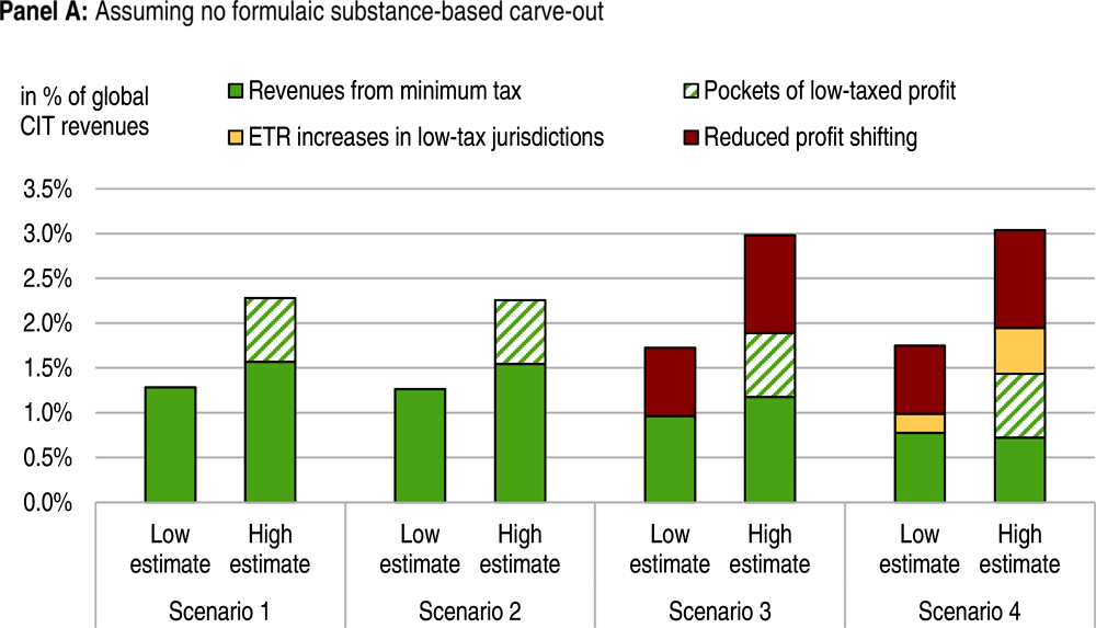
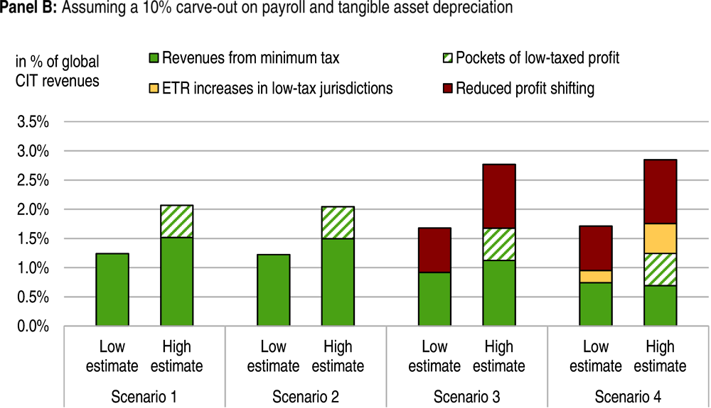
Note: Scenario 1 is a static scenario without behavioural reactions. Scenario 2 takes into account the interaction of Pillar Two with Pillar One. Scenario 3 adds the reaction of MNEs in the form of lower profit shifting intensity. Scenario 4 adds the reaction of governments, in the form of some jurisdictions with an ETR below the minimum rate increasing their ETR to the minimum rate. The results focus illustratively on a scenario assuming a 12.5% minimum rate, with no formulaic substance-based carve-out (Panel A) or a 10% carve-out on payroll and tangible asset depreciation (Panel B). Consistent with the assumption that GILTI would coexist with Pillar Two, the estimates in these figures exclude revenues gains related to MNEs with an ultimate parent in the United States. The ranges between low and high estimates reflect data uncertainty, and the upper bound of the ranges also takes into account uncertainty related to pockets of low-taxed profit in higher-tax jurisdictions.
Source: OECD Secretariat.
3.9.3. Revenue gains for broad jurisdiction groups
278. Results by broad jurisdiction groups across the four scenarios and for several illustrative minimum tax rates (10%, 12.5% and 15%) are presented in Figure 3.13. The results exclude revenue gains related to US MNEs, and the group of high income jurisdictions excludes the United States. Panel A includes all four groups considered in the analysis (high, middle and low income, and investment hubs), while Panel B presents the same results excluding investment hubs (Panel A). Excluding investment hubs makes it possible to use a different scale and increases the readability of the results for the other groups.
279. High, middle and low income jurisdictions would gain revenues from Pillar Two under all four scenarios considered. Revenue gains tend to be larger among high income jurisdictions than lower income ones, reflecting that most MNE group ultimate parents are located in high income jurisdictions, implying that gains from the IIR primarily accrue to these jurisdictions. Still, gains in middle and low income jurisdictions are also significant, especially once the reduced profit shifting intensity of MNEs is taken into account (Scenarios 3 and 4).
280. Investment hubs would gain revenues in Scenarios 1 and 2, while they would gain less revenues on average in Scenario 3. They could even lose revenues in this scenario, depending on the level of the minimum tax rate (Figure 3.13, Panel A). This is because reduced MNE profit shifting would reduce the size of the tax base in a number of investment hubs where profit is currently shifted. However, the magnitude of this average revenue loss is difficult to measure with precision, as it depends on the effective tax rate on this shifted profit. The loss may be compounded by potential knock-on effects of reduced investment in investment hubs on other tax bases, which are not taken into account in the estimates. Also, it is important to note that results vary across investment hubs, which are a relatively heterogeneous group. Finally, in Scenario 4, investment hubs would on average benefit from relatively large revenue gains, reflecting the assumption that a number of them would increase their ETR on low-taxed profit. As investment hubs capture a higher share of global revenue gains, gains in other jurisdiction groups tend to be lower in Scenario 4 than in Scenario 3.
281. Results for hybrid scenarios taking into account MNE and government reactions (as in Scenarios 3 and 4) but not the interaction with Pillar One are presented in Annex 3.B and are qualitatively similar to the results in Figure 3.13. The results in Figure 3.13 assume illustratively a 10% carve-out on payroll and tangible asset depreciation. Results in a scenario without a formulaic substance-based carve-out are presented in Annex 3.E. They are also qualitatively similar to Figure 3.13, but revenue gains across all groups are slightly higher than in the scenario with a carve-out.

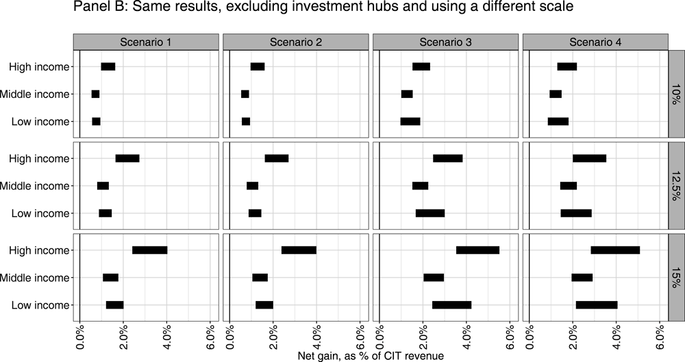
Note: Each facet in the figure correspond to one of four scenarios (in columns) and one of three illustrative minimum tax rates (in rows). Results in Panel B are identical to results in Panel A, except that the investment hubs group is excluded, which makes it possible to use a different scale and increases the readability of results for the other groups. Scenario 1 is a static scenario without behavioural reactions. Scenario 2 takes into account the interaction of Pillar Two with Pillar One. Scenario 3 adds the reaction of MNEs in the form of lower profit shifting intensity. Scenario 4 adds the reaction of governments, in the form of some jurisdictions with an ETR below the minimum rate increasing their ETR to the minimum rate. The results focus illustratively on a scenario with a 10% carve-out on payroll and tangible asset depreciation (results without carve-out are presented in Annex 3.E). Groups of jurisdictions (high, middle and low income) are based on the World Bank classification. Investment hubs are defined as jurisdictions with a total inward FDI position above 150% of GDP. The high income group excludes the United States, in light of the illustrative assumption that GILTI would coexist with Pillar Two. The ranges reflect data uncertainty, and the upper bound of the ranges also takes into account uncertainty related to pockets of low-taxed profit in higher-tax jurisdictions.
Source: OECD Secretariat.
282. This chapter describes the methodology and data sources used by the OECD Secretariat to estimate the order of magnitude of potential tax revenue implications of Pillar Two, across a range of illustrative Pillar Two design and parameter options and under stylised assumptions regarding potential behavioural reactions by MNEs and governments. The chapter also presents the estimated revenue gains at the global level and for broad jurisdiction groups.
283. As discussed in Chapter 1, jurisdiction-level results have been shared on a confidential and bilateral basis with most Inclusive Framework members. The OECD Secretariat has provided estimates to more than 115 jurisdictions at their request. Jurisdiction-specific results were shared in the form of revenue estimation ‘tools’. These tools provide jurisdictions with the ability to consider the estimated impact on tax revenues in their jurisdiction of a range of potential Pillar Two parameters (e.g. minimum tax rate, carve-out percentage). Estimates in the tools are presented as ranges to reflect the data uncertainty. After extensive consultation with members of the Inclusive Framework, there was no consensus over whether or not jurisdiction-specific estimates should be publicly released as part of the economic impact assessment. In view of this lack of consensus, no jurisdiction-specific estimates are included in this chapter.
284. The results in this chapter suggest that revenue gains from Pillar Two could be significant across all groups of jurisdictions. Pillar Two would likely reduce MNE profit shifting intensity, which would yield additional tax revenue gains supplementing the direct gains from the minimum tax in many jurisdictions. The interaction of Pillar One with Pillar Two would reduce estimated Pillar Two gains only at the margin. The estimated gains from Pillar Two depend substantially on the minimum tax rate considered, while the effect of the formulaic substance-based carve-out modelled in this chapter on the estimated gains is relatively small. Finally, the distribution of revenue gains across jurisdictions depends on potential government reactions, and in particular on whether governments in some low-tax jurisdictions would increase their ETR in reaction to the introduction of Pillar Two.
285. As discussed in the introduction and throughout the chapter, the estimates rely on a number of simplifying assumptions about Pillar Two design and in the modelling of behavioural reactions to Pillar Two. Behavioural reactions are always difficult to anticipate, especially in an area as complex as MNE profit shifting behaviour. Finally, the data underlying the analysis have a number of limitations. In particular, it inevitably predates the COVID-19 crisis, as well as other important developments such as the implementation of various measures under the OECD/G20 BEPS project and the introduction of the US Tax Cuts and Jobs Act (TCJA). Many key results in this chapter can be expected to remain valid in the post-COVID-19 environment (e.g. on the sensitivity of the outcomes to the various Pillar Two parameter choices, or the implications of the behavioural reactions considered). However, as the profitability of many MNEs is likely to be substantially reduced by the crisis in the short to medium term, the crisis could reduce potential gains from Pillar Two at this horizon. The longer term implications of the crisis for Pillar Two revenue gains will depend on the structural economic changes that the crisis may bring or accelerate, which remain largely uncertain at this stage.
References
[12] Beer, S., R. de Mooij and L. Liu (2019), “International Corporate Tax Avoidance: A Review of the Channels, Magnitudes, and Blind Spots”, Journal of Economic Surveys, pp. 1-29, https://doi.org/10.1111/joes.12305.
[18] Bilicka, K. (2019), “Comparing UK Tax Returns of Foreign Multinationals to Matched Domestic Firms”, American Economic Review, Vol. 109/8, pp. 2921-2953, https://doi.org/10.1257/aer.20180496.
[7] Blouin, J. and L. Robinson (2019), “Double Counting Accounting: How Much Profit of Multinational Enterprises Is Really in Tax Havens?”, SSRN Electronic Journal, https://doi.org/10.2139/ssrn.3491451.
[11] Bradbury, D., T. Hanappi and A. Moore (2018), “Estimating the fiscal effects of base erosion and profit shifting: data availability and analytical issues”, Transnational Corporations, Vol. 25/2, https://dx.doi.org/10.18356/e1d7a8b4-en.
[8] Clausing, K. (2020), “Profit Shifting Before and After the Tax Cuts and Jobs Act”, SSRN Electronic Journal, https://doi.org/10.2139/ssrn.3274827.
[27] Clifford, S. (2019), “Taxing multinationals beyond borders: Financial and locational responses to CFC rules”, Journal of Public Economics, Vol. 173, pp. 44-71, https://doi.org/10.1016/j.jpubeco.2019.01.010.
[13] Cobham, A., T. Faccio and V. FitzGerald (2019), “Global inequalities in taxing rights: An early evaluation of the OECD tax reform proposals”, SocArXiv Papers, https://doi.org/10.31235/osf.io/j3p48.
[22] Cobham, A. and P. Janský (2018), “Global distribution of revenue loss from corporate tax avoidance: re-estimation and country results”, Journal of International Development, Vol. 30/2, pp. 206-232, https://doi.org/10.1002/jid.3348.
[28] Damgaard, J., T. Elkjaer and N. Johannesen (2019), “What Is Real and What Is Not in the Global FDI Network?”, IMF Working Papers, Vol. 19/274, https://doi.org/10.5089/9781513521527.001.
[10] Devereux, M. et al. (2020), The OECD Global Anti-Base Erosion (“GloBE”) proposal, https://www.sbs.ox.ac.uk/sites/default/files/2020-02/OECD_GloBE_proposal_report.pdf.
[20] Dowd, T., P. Landefeld and A. Moore (2017), “Profit shifting of U.S. multinationals”, Journal of Public Economics, Vol. 148, pp. 1-13, https://doi.org/10.1016/j.jpubeco.2017.02.005.
[21] Fuest, C., S. Hebous and N. Riedel (2011), “International debt shifting and multinational firms in developing economies”, Economics Letters, Vol. 113/2, pp. 135-138, https://doi.org/10.1016/j.econlet.2011.06.012.
[23] Heckemeyer, J. and M. Overesch (2017), “Multinationals’ profit response to tax differentials: Effect size and shifting channels”, Canadian Journal of Economics/Revue canadienne d’économique, Vol. 50/4, pp. 965-994, https://doi.org/10.1111/caje.12283.
[14] Hines, J. and E. Rice (1994), “Fiscal Paradise: Foreign Tax Havens and American Business”, The Quarterly Journal of Economics, Vol. 109/1, pp. 149-182, https://doi.org/10.2307/2118431.
[26] Horst, T. (2019), “Preliminary Esmates of the Likely Actual Revenue Effects of the TCJA’s Provisions”, Tax Notes International, http://www.horstfrisch.com/pdf/003.pdf.
[17] Huizinga, H. and L. Laeven (2008), “International profit shifting within multinationals: A multi-country perspective”, Journal of Public Economics, Vol. 92/5-6, pp. 1164-1182, https://doi.org/10.1016/j.jpubeco.2007.11.002.
[19] Johannesen, N., T. Tørsløv and L. Wier (2019), “Are Less Developed Countries More Exposed to Multinational Tax Avoidance? Method and Evidence from Micro-Data”, The World Bank Economic Review, Vol. 2019, pp. 1-20, https://doi.org/10.1093/wber/lhz002.
[25] Johansson, Å. et al. (2017), “Tax planning by multinational firms: Firm-level evidence from a cross-country database”, OECD Economics Department Working Papers, No. 1355, OECD Publishing, Paris, https://doi.org/10.1787/9ea89b4d-en.
[3] Keen, M. and K. Konrad (2013), “The theory of international tax competition and coordination”, Handbook of Public Economics, Vol. 5, pp. 257-328, https://doi.org/10.1016/B978-0-444-53759-1.00005-4.
[6] OECD (2020), “Anonymised and aggregated Country-by-Country Report statistics”, Corporate Tax Statistics - Second Edition, OECD Publishing, https://www.oecd.org/tax/beps/corporate-tax-statistics-database.htm.
[9] OECD (2020), “Corporate Tax Statistics - Second Edition”, OECD Publishing, https://www.oecd.org/tax/tax-policy/corporate-tax-statistics-second-edition.pdf.
[1] OECD (2020), Tax Challenges Arising from Digitalisation – Report on Pillar Two Blueprint: Inclusive Framework on BEPS, OECD/G20 Base Erosion and Profit Shifting Project, OECD Publishing, Paris, https://dx.doi.org/10.1787/abb4c3d1-en.
[24] OECD (2015), Measuring and Monitoring BEPS, Action 11 - 2015 Final Report, OECD/G20 Base Erosion and Profit Shifting Project, OECD Publishing, Paris, https://dx.doi.org/10.1787/9789264241343-en.
[15] Tørsløv, T., L. Wier and G. Zucman (2019), “The Missing Profits of Nations: 2017 Figures”, https://missingprofits.world/wp-content/uploads/2020/04/TWZUpdate.pdf.
[16] Tørsløv, T., L. Wier and G. Zucman (2019), The Missing Profits of Nations: Updated Figures, https://missingprofits.world/wp-content/uploads/2019/09/TWZUpdate.pdf.
[5] Tørsløv, T., L. Wier and G. Zucman (2018), “The Missing Profits of Nations”, NBER Working Paper, No. 24701, http://www.nber.org/papers/w24701.pdf.
[2] US Joint Committee on Taxation (2017), Estimated budget effects of the conference agreement for H.R. 1, the “Tax Cuts and Jobs Act”, JCX-67-17, https://www.jct.gov/publications.html?func=startdown&id=5053.
[4] von Schwerin, A. and T. Buettner (2016), Constrained Tax Competition – Empirical Effects of the Minimum Tax Rate on the Tax Rate Distribution, Annual Conference 2016: Demographic Change, German Economic Association, http://hdl.handle.net/10419/145642.
286. The results in Scenarios 2-4 of this chapter take into account how the interaction with Pillar One would affect Pillar Two results. This annex presents alternative results ignoring the effect of this interaction. Overall, these results are very close to the results taking the interaction into account, reflecting that the effect of this interaction is small under the assumptions on Pillar One and Pillar Two design and parameters considered this chapter.

Note: The light blue intervals correspond to the Pillar Two results presented in the main text, which take into account the interaction with Pillar One (see for example Figure 3.13). The dark blue intervals do not take this interaction into account, and can therefore be interpreted as the effect of Pillar Two if it were implemented in isolation. For simplicity, the results focus illustratively on a scenario with no formulaic substance-based carve-out. Only Scenario 3 and Scenario 4 are presented (without Pillar One interaction, Scenario 2 is identical to Scenario 1, which is presented in the main text of this chapter). The high income group excludes the United States, in light of the illustrative assumption that GILTI would coexist with Pillar Two. The ranges reflect data uncertainty, and the upper bound of the ranges also takes into account uncertainty related to pockets of low-taxed profit in higher-tax jurisdictions.
Source: OECD Secretariat.
287. Measures of economic activity are required in two parts of the analysis: (i) as proxy measures to allocate potential revenue gains from the undertaxed payments rule (UTPR), and (ii) as proxy measures to assess where shifted profit originates in the modelling of MNE profit shifting. In both cases, the baseline results in this chapter are relying on turnover as a measure of economic activity. Turnover data are sourced from the turnover matrix described in Chapter 5. Alternative results based on tangible assets or payroll are presented in this annex. The data for tangible assets and payroll are sourced from similar matrices, also described in Chapter 5.
288. The results in this annex focus first on the sensitivity of results to the proxy used for the allocation of gains from the UTPR (Annex Table 3.C.1 and Annex Figure 3.C.1) and second on the sensitivity of results to the proxy used for the profit shifting modelling (Annex Table 3.C.2 and Annex Figure 3.C.2). Overall, results are not very sensitive to these different modelling assumptions.
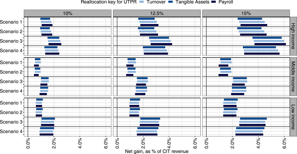
Note: This figure presents Pillar Two estimates by jurisdiction groups, illustrating the implications of using different measures of economic activity to proxy for the allocation of UTPR revenues: turnover (as in the baseline results), tangible assets and payroll. Scenario 1 is a static scenario without behavioural reactions. Scenario 2 takes into account the interaction of Pillar Two with Pillar One. Scenario 3 adds the reaction of MNEs in the form of lower profit shifting intensity. Scenario 4 adds the reaction of governments, in the form of some jurisdictions with an ETR below the minimum rate increasing their ETR. The results focus illustratively on a scenario with no carve out. Investment hubs are excluded to enhance readability of results for the other groups. The high income group excludes the United States, in light of the illustrative assumption that GILTI would coexist with Pillar Two. The ranges reflect data uncertainty, and the upper bound of the ranges also takes into account uncertainty related to pockets of low-taxed profit in higher-tax jurisdictions.
Source: OECD Secretariat.

Note: The results in this figure present the sensitivity of estimated Pillar Two gains in Scenario 3 and Scenario 4, to using alternative proxies for economic activity to assess the origin of MNE shifted profits. Baseline results in this chapter are based on turnover (i.e. assume that MNE profit originates in jurisdictions where MNEs shifting profit have turnover), and alternative results in this figure focus on tangible assets and payroll. The profit shifting modelling methodology is the same as described in this chapter, except for the proxy used to assess profit origin. Only Scenario 3 and Scenario 4 are included as Scenarios 1 and 2 do not depend on the profit shifting modelling. The results focus illustratively on a scenario with no carve out. The high income group excludes the United States, in light of the illustrative assumption that GILTI would coexist with Pillar Two. The ranges reflect data uncertainty, and the upper bound of the ranges also takes into account uncertainty related to pockets of low-taxed profit in higher-tax jurisdictions.
Source: OECD Secretariat.
289. Jurisdiction-level effective tax rates (ETR) play an important role in the assessment of Pillar Two revenue gains since they are the rates that are compared to the minimum tax, and which can be increased in Scenario 4. They are also included in the tax rate differentials used to assess the origin of shifted profits and the reduction implied by the minimum tax. In the baseline analysis, the average ETR on MNE profit in a jurisdiction is measured as the median estimate obtained across three data sources (see Section 3.4.2) including data from anonymised and aggregated CbCRs.
290. The results in this annex focus on the sensitivity of results to the exclusion of CbCR as a data source on ETRs. Overall, the results suggest that this exclusion would lead to lower estimates of Pillar Two gains, but without changing the broad order of magnitude of the results.

Note: The results in this figure present the sensitivity of estimated Pillar Two gains to excluding CbCR as a source when computing the jurisdiction-level ETRs used in the analysis. Baseline results in this chapter compute ETRs by taking the median of three sources (Tørsløv et al. (2018[5]), US BEA data and CbCR data). The robustness check excludes the data from CbCRs from this calculation. The results focus illustratively on a scenario with no carve out. The high income group excludes the United States, in light of the illustrative assumption that GILTI would coexist with Pillar Two. The ranges reflect data uncertainty, and the upper bound of the ranges also takes into account uncertainty related to pockets of low-taxed profit in higher-tax jurisdictions.
Source: OECD Secretariat.

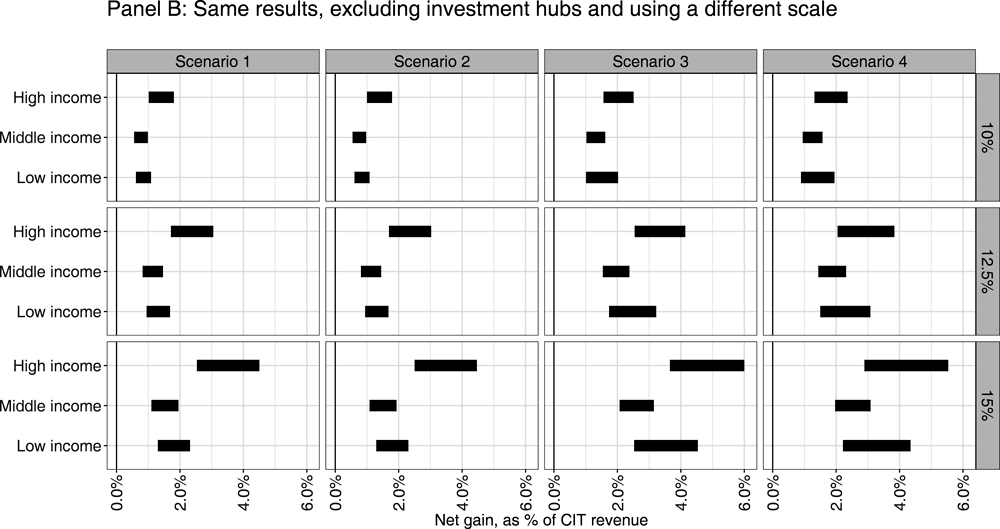
Note: This figure is identical to Figure 3.13, with the difference that it assumes no formulaic substance-based carve out (while Figure 3.13 assumes a 10% carve-out on payroll and tangible asset depreciation). Scenario 1 is a static scenario without behavioural reactions. Scenario 2 takes into account the interaction of Pillar Two with Pillar One. Scenario 3 adds the reaction of MNEs in the form of lower profit shifting intensity. Scenario 4 adds the reaction of governments, in the form of some jurisdictions with an ETR below the minimum rate increasing their ETR. The high income group excludes the United States, in light of the illustrative assumption that GILTI would coexist with Pillar Two. The ranges reflect data uncertainty, and the upper bound of the ranges also takes into account uncertainty related to pockets of low-taxed profit in higher-tax jurisdictions.
Source: OECD Secretariat.
Notes
← 1. In all this chapter, low-tax jurisdictions refers to jurisdictions with an average ETR below the minimum rate (and a variety of potential minimum rates are illustratively considered in this chapter), and higher-tax jurisdictions refers to jurisdictions with an average ETR above the minimum rate.
← 2. The OECD/G20 BEPS Package was released in October 2015 and various measures outlined in the package have been implemented in the years that have followed. A range of measures agreed to be implemented by members of the Inclusive Framework continue to be implemented by jurisdictions and, therefore, the full effect of these measures is not captured in the data available at the time of this analysis.
← 3. For example, CbCR data, which is an important data source for the analysis, focuses only on one year (2016) and contains no information on whether profit-making MNE sub-groups in a jurisdiction in 2016 have been in a loss position in that jurisdiction in the previous years.
← 4. In presence of a formulaic substance-based carve-out, an ETR increase in a low-tax jurisdiction could slightly increase the overall tax payments of an MNE group as it would lose the benefit of the carve-out on the profit in this low-tax jurisdiction. However, as further discussed below, this effect is quantitatively small under the parameters considered in this chapter.
← 5. If one assumes a non-cooperative simultaneous rate setting (Nash equilibrium), the introduction of a minimum tax rate tends to lead the higher-tax jurisdiction to increase its rate, while under a sequential rate setting system where the higher-tax jurisdiction is a Stackelberg leader, the higher-tax jurisdiction tends to reduce its rate when the minimum tax is introduced (Keen and Konrad, 2013[3]). In a simultaneous game, the best “response” (in terms of tax rate) of a jurisdiction is usually to increase its tax rate when other jurisdictions’ increase their rates, since if the other jurisdictions have higher tax rates, a jurisdiction can increase its own rate to increase revenue without losing its attractiveness. The introduction of a minimum tax tends to increase the “best response” rate of jurisdictions above the minimum tax in this setting. In a sequential game, the first mover takes into account that setting a low tax rate might not be beneficial since the followers can decrease their own. With a minimum tax rate, this “threat” from followers is weaker.
← 6. There are two important limitations with CbCR data: (i) there are inconsistencies in the way dividends from affiliates are reported (i.e. sometimes included and sometimes not), and (ii) certain jurisdictions report profit for “stateless” entities, which may correspond to different situations, including “pass-through” entities (see Box 3 in OECD (2020[6]) and https://www.oecd.org/tax/tax-policy/anonymised-and-aggregated-cbcr-statistics-disclaimer.pdf). Reflecting this, the profit of “stateless” entities is not included in the profit matrix. Extensive benchmarking of CbCR data against other sources (e.g. ORBIS) suggests that these issues do not alter substantially the overall picture, as further discussed in Chapter 5.
← 7. The amount of losses of loss-making MNE sub-groups in a given year does not clearly indicate how large the effect of a potential loss carry-forward mechanism under Pillar Two would be. For example, it is possible that some MNE sub-groups are persistently in a profit position in a jurisdiction (and therefore never benefit from any loss carry-forward) while others are persistently in a loss position (and never have a Pillar Two liability against which to use their carried-forward losses).
← 8. For example, if profit-making sub-groups make a profit of 100 and pay taxes of 20, while loss-making sub-groups make a loss of 15 and pay no taxes, the average ETR of profit-making sub-groups is 20/100=20%, while the average ETR computed across profit-making and loss-making sub-groups is 20/(100-15)=24%. An ETR focusing only on profit-making sub-groups would be more consistent with the Pillar Two analysis in this chapter.
← 9. This methodology focusing on foreign taxes and profits of US MNEs is used to compute ETRs in jurisdictions other than the United States. To complement this, an average ETR of (foreign-owned) MNEs in the United States is computed using the same methodology applied to the BEA data on foreign direct investment in the United States.
← 10. These other sources are The International Bureau of Fiscal Documentation, and publicly available tax rates from KPMG, EY, and the Tax Foundation.
← 11. The estimated gains also take into account the jurisdiction-specific assumptions on Pillar Two implementation described in section 3.4.5, which result in a small share of low-taxed profit not being subject to the top-up tax.
← 12. For example, if about 20% of profit in higher-tax jurisdictions is estimated to be carved out, the upper bound of the Pillar Two uncertainty range is increased by 40% (i.e. 50%*(1-20%)) instead of 50%.
← 13. These figures are based on the estimates of global CIT revenues in Devereux et al. (2020[10]), which are lower than those in this report due to less extensive geographic coverage and the focus on an earlier year of reference.
← 14. In ORBIS, coverage of tangible assets (which is the variable used as a basis to approximate depreciation expenses) is generally better than coverage of payroll.
← 15. Indeed, while it is relatively straightforward to compute directly the effect of a combined carve-out with firm-level data in jurisdictions where these data are available, it is more difficult to do it in the jurisdictions where only aggregate data are available.
← 16. For example, if the profit of an MNE sub-group is EUR 15, its payroll EUR 100 and its depreciation expenses EUR 100, then a 10% payroll carve-out would carve out an amount of EUR 10 and a 10% depreciation carve-out would also carve out an amount of EUR 10. Summing the two would suggest a total carve-out effect of EUR 20, while the combined carve-out would only carve out an amount of EUR 15 (i.e. the total profit of the sub-group).
← 17. The US BEA provides detailed data on depreciation by asset classes in the private sector without distinguishing MNE entities from non-MNE entities (the BEA database on the activity of US MNEs also provides data on depreciation, but does not distinguish between tangible and intangible assets). When considering private non-residential fixed assets (i.e. ‘equipment’ and ‘structures’), the ratio of depreciation expenses to the stock of tangible assets, estimated at current cost, is stable around 6.3-6.5% between 2011 and 2018. Disaggregation by industry at the 2-digit NAICS code suggests heterogeneity across sectors, with the average depreciation rate ranging between 2.6% (real estate and rental and leasing), and 12.7% (construction). One caveat on those numbers is that depreciation in national accounts can differ from depreciation in tax and financial accounts. Table 7.13 of the National Income and Product Accounts relates depreciation and amortisation as reported by the US Internal Revenue Service and as included in the national accounts, and suggests that most of the differences come from a different treatment of intangible assets. Another source of information on depreciation is the balance sheet and income statement data available in ORBIS. ORBIS data contains firm-level information on depreciation of assets, but without distinction between the depreciation of tangible fixed assets and the amortisation of intangible fixed assets. On average, for domestic and multinational firms included in ORBIS, the ratio of depreciation and amortisation on total (tangible and intangible) fixed assets was around 5.8% over the past two decades. Given that tangible fixed assets represent around half of total fixed assets and that the amortisation rate of intangible assets is likely higher than the depreciation rate of tangible assets, this suggests that 10% is indeed an upper bound for the average depreciation rate of tangible fixed assets.
← 18. Assuming a linear relationship implies that, above a certain level of the aggregate profitability ratio, no profit at all would be carved-out which is not completely realistic. However, a robustness check assuming that at least a minimum percentage of profit (e.g. 1%) would be carved-out in all jurisdictions suggests that this has little effect on the overall results (i.e. reduction of total Pillar Two revenue gains by less than 2%).
← 19. The assumptions on the upper bound of the range to take into account uncertainty related to pockets of low-taxed profit are the following: +50% in a no carve-out scenario (as discussed in Section 3.4.3), +45% when the carve-out percentage is 5%, +40% when the carve-out percentage is 10%, +35% when the carve-out percentage is 15% and +30% when the carve-out percentage is 20%. These assumptions aim to be relatively simple and at the same time consistent with estimates of the share of carved-out profit in higher-tax jurisdictions. For example, with a 10% carve-out percentage, 16-19% of profit in higher-tax jurisdictions is estimated to be carved-out (see Table 3.5). In turn, assuming that 20% of profit in higher-tax jurisdictions is carved out would lead to an increase in the upper bound of the uncertainty range by 40% (i.e. 50%*(1-20%)) instead of 50% in the no-carve-out scenario.
← 20. As discussed above, the United States is an exception, as it is assumed in this chapter that GILTI would coexist with Pillar Two and that the United States would apply GILTI (instead of an income inclusion rule) to MNEs with an ultimate parent in the United States (see Section 3.8).
← 21. As discussed above, the switch-over rule and the subject to tax rule would also contribute to bringing the ETR on low-taxed profit up to the level of the minimum rate, but they are not modelled in this chapter due to data limitations.
← 22. An alternative approach would be to use bilateral FDI data (e.g. on royalty and interest flows) to identify transactions that may be subject to the UTPR. This may be closer to the actual spirit of the UTPR, but poses other methodological challenges, related to the potential double counting of flows that are channelled through several jurisdictions, as well as data gaps in bilateral FDI flow statistics (see Annex 5.C of Chapter 5).
← 23. MNE turnover in certain jurisdictions can be inflated as a result of tax planning strategies. To avoid that this has a disproportionate effect on the results, MNE turnover is capped at 100% of GDP in all jurisdictions.
← 24. In practice, the amount of residual profit relieved under Pillar One is computed for each pair of jurisdictions in the profit matrix in Chapter 2, while the amount of residual profit received is only computed at the level of each receiving jurisdiction (rather than bilaterally). To disaggregate the amount of received residual profit received on a bilateral basis, it is assumed that the residual profit in each column (i.e. each jurisdiction of ultimate parent) is redistributed according to the same distribution key used for the reallocation of the global residual profit in Chapter 2, that is based on the geographical distribution of destination-based sales. This approach ensures that the aggregate numbers obtained in the estimation are consistent with the Pillar One estimates obtained in Chapter 2.
← 25. For practical reasons, jurisdictions are either considered as profit origin or as profit destination in this chapter, but not both.
← 26. On the link between high FDI positions and profit shifting, see for example Damgaard et al. (2019[28]).
← 27. This is because profits shifted to jurisdictions where the average ETR is above the minimum rate would generally not be subject to Pillar Two. However, situations where the ETR on this shifted profit would be below the minimum rate could arise (and these profits would be subject to Pillar Two) due to the existence of pockets of low-taxed profits in higher-tax jurisdictions.
← 28. It is possible that reduced incentives to shift profit to jurisdictions with an average ETR below the minimum rate could increase MNEs’ willingness to shift profit to jurisdictions with an average ETR above the minimum rate. This possibility is not modelled in this chapter, as there is no clear way to identify the magnitude of this effect and the jurisdictions where more profit would be shifted without more granular data on the cost of shifting profit to different jurisdictions.
← 29. Other profitability ratios could be considered to define “normal” profit (e.g. profit to total assets). The ratio of profit to turnover was chosen because it could be easily computed across all pairs of jurisdictions based on the data available in the profit and the turnover matrices.
← 30. This estimate includes MNEs with an ultimate parent in the United States, for the purpose of comparability with estimates from the economic literature.
← 31. On the data sources underlying the turnover matrix and its construction, see Chapter 5.
← 32. In contrast, Johansson et al. (2017[25]) tend to find a lower average tax rate semi-elasticity vis-à-vis zero-tax jurisdictions than among jurisdictions with strictly positive tax rates.
← 33. This aggregate semi-elasticity is obtained by dividing the share of shifted profits in total profits (observed and shifted) in “profit origin” jurisdictions (12.5%), by the average statutory tax rate differential between “profit origin” jurisdictions and “profit destination” jurisdictions (10.3 percentage points). These tax rates are weighted by turnover. While this chapter uses a combination of statutory and effective tax rates to model profit shifting, this calculation is based exclusively on statutory tax rates for comparability with the literature (which generally relies on statutory rates). The semi-elasticity is estimated with a degree of uncertainty, as it depends among other things on the assumptions on the “normal” profitability level considered, the shape of the relationship between profit shifting and tax rate differentials, or the weights used to aggregate the coefficients.
← 34. In presence of a formulaic substance-based carve-out, an ETR increase in a low-tax jurisdiction could result in a slightly higher amount of tax due by an MNE because it would lose the benefit of the substance carve-out included in Pillar Two. However, as further discussed below, this effect is quantitatively small.
← 35. For example, Clifford (2019[27]) finds that in response to CFC rules, MNEs redirect profits from subsidiaries below the CFC ‘low-tax’ threshold into subsidiaries just above the threshold and change incorporation patterns to place fewer subsidiaries below and more above the threshold. Roughly half of the resulting increase in global tax revenue is found to accrue to the rule-enforcing jurisdiction.
← 36. This assumption would not be valid if the ETR calculation rules in the presence of a carve-out would not require MNEs to make an adjustment to the covered taxes associated with the carved-out profit.
← 37. This calculation assumes illustratively a 12.5% minimum tax rate and a 10% carve-out percentage. The reduction in profit shifting is also very small with other assumptions on the minimum tax and carve-out rates considered in this chapter.
← 38. For example, relocating employees representing USD 10 million of payroll into a zero-tax jurisdiction would offer a carve-out of USD 1 million (assuming a 10% carve-out rate), which if used in full would reduce the amount of tax paid under Pillar Two by USD 0.125 million (assuming a 12.5% minimum tax rate). This tax saving seems unlikely to justify the cost of relocation.
← 39. This is because the factors that contribute to differences between statutory and effective rates (e.g. depreciation rules, tax deductions, tax credits) are generally linked to real economic activity.
← 40. The difference with the reasoning in the previous endnote is that shifted profit may benefit from preferential treatment in “profit destination” jurisdictions, and that the resulting ETR may essentially reflect this preferential treatment, without necessarily being related to the level of the statutory rate in these jurisdictions.
← 41. For example, one can consider an MNE group that has a profit of EUR 100, payroll of EUR 40, depreciation expenses of EUR 10, and paid zero tax in a certain jurisdiction. Under Pillar Two, assuming a 12.5% minimum tax rate and a 10% carve-out rate, the MNE would have to pay 12.5%*(100-10%*(40+10))= EUR 11.9. If the jurisdiction increases the ETR of this MNE to 12.5%, the MNE would have to pay this rate on all of its profit (EUR 100), which would result in a tax of 12.5%*100= EUR 12.5, which is higher than the EUR 11.9 paid before the ETR increase.
← 42. If jurisdictions increasing their ETRs want to preserve neutrality for the overall amount of tax paid of MNEs, they might try to mimic the functioning of Pillar Two in their tax system, by applying an ETR increase including a carve-out provision that would have the same design and mark-up percentage as the formulaic substance-based carve-out in Pillar Two. In practice however, such a mechanism may not necessarily be straightforward to design or to make consistent with other features of a jurisdiction’s corporate tax system.
← 43. For MNEs having an average ETR on their foreign profit that is above the GILTI rate (and therefore not paying taxes under GILTI), an ETR increase in a zero-tax jurisdiction would fully translate into an overall tax increase. For MNEs with an average ETR below the GILTI rate, an ETR increase in a zero-tax jurisdiction would also result in an overall tax increase since only 80% of foreign taxes are credited under GILTI in that situation. In that case, the overall tax increase would represent 20% of the liability arising from the ETR increase.
← 44. Jurisdictions in this group may consider increasing the ETR on the pockets of low-taxed profit in their jurisdiction if there are some. For simplicity and due to lack of data on these pockets, this potential reaction is not considered in this chapter.
← 45. Companies face a US tax liability at a 10.5% rate on the relevant income and a non-refundable tax credit on 80% of foreign taxes paid. If the foreign ETR is 13.125% or above, the tax credit covers the whole US tax liability. By the same logic, the US tax liability at 13.125% starting in 2026 with the same tax credit yields an upper bound of 16.40625%. These are the tax rates determined applying the statutory GILTI rules and do not take into account other features of the US international tax system, such as expense allocation, that may effectively increase a specific taxpayer’s overall US tax liability by limiting the creditability of foreign taxes.
← 46. A first assessment of the impact of GILTI on profit shifting has been produced by Clausing (2020[8]). She estimates that GILTI could “reduce the corporate profits of US multinational affiliates in ‘haven’ countries by about 12 to 16 percent”, which could bring “an 8 to 9 percent increase in the US entity corporate tax base in foreign jurisdictions above the minimum tax threshold, and a USD 15-30 billion increase in the US corporate tax base each year.” However, these results are highly sensitive to the assumptions on the share of US MNEs that have an average ETR on their foreign profit above or below the GILTI rate (see Appendix C in Clausing (2020[8])).
← 47. Global revenue gains in Scenarios 3 and 4 are similar, reflecting that the reaction modelled in Scenario 4 primarily changes the distribution of these gains across jurisdictions. Still, there is a slight increase in global revenue gains between Scenarios 3 and 4. This comes from two reasons. First, the ETR increases in Scenario 4 reduce the (relatively small) amount of global low-taxed profit that is not fully taxed under Pillar Two under the assumptions considered in this chapter (see Section 3.7.1 above). For example, this would be the case for the profit in an MNE entity located in a jurisdiction from Group 3 (which would increase its ETR under Scenario 4), if this MNE has an ultimate parent in a jurisdiction from Group 2 (which does not apply an IIR) and its economic activity also in a jurisdiction from Group 2 (which does not apply a UTPR). Second, the ETR increases imply that some low-taxed profit that benefitted from a formulaic substance-based carve-out under Pillar Two would be taxed, leading to larger revenue gains overall.