copy the linklink copied! Chapter 2. Changing the lens: Development beyond income
This chapter illustrates the weakness of income per capita as a measure of development in Latin America and the Caribbean. Trends in income per capita may not fully reflect changes in other dimensions of development. Countries with similar levels of income per capita display very different development outcomes. This is especially true for those that are middle- and upper middle-income, such as most Latin American and Caribbean countries. This chapter compares current and long-term trends in income per capita with other well-being indicators at regional, national and sub-national levels. It also discusses the importance of developing adapted statistics that better reflect people’s living standards to improve the design, implementation and monitoring of public policy for development.

copy the linklink copied! Introduction
This chapter provides evidence of the imperfect relationship between income per capita and a range of development outcomes through a series of exploratory analyses. This evidence shows clearly that income per capita and other development outcomes do not always move in sympathy.
There is no standard definition of development. Different actors have continuously argued about their preferred development objectives, such as economic growth, social welfare, political participation, freedom, national independence and environmental integrity. While theorists have favoured some objectives over others at different periods, development strategies have increasingly come to embrace all of them (De Janvry and Sadoulet, 2014).
Development paradigms are the result of external factors and accumulated knowledge. External factors have indeed played a major role in shifting paradigms. The era of economic planning in the 1960s, when economic development was treated as a precise science, demonstrated that development was more than just about the economy. Already in the 1970s, the need to look beyond gross domestic product (GDP) was brought to the fore of development thinking and practice (Seers, 1969). In 1972, the Stockholm Conference on the Human Environment was an important milestone in environmental policy making at the global level, while the 1995 World Summit on Social Development was pivotal on the social side. Both strands were reflected in the 1987 Brundtland Report and the 1992 Earth Summit.
Economic structure and its transformation matter. It was commonly thought that developing countries would have to follow a different path from previously industrialising ones. This view was advocated by the dependency school, for example (Prebisch, 1949). But the oil crisis in 1973 and the debt crises in Latin America a few years later placed macro-stability front and centre for the next two decades.
Today’s theorists have built on a vast array of earlier development thinking. They have come up with more holistic approaches, including addressing environmental and climate issues in ways that reflect local conditions, and addressing people’s needs and wants (OECD, 2018a).
A consensus is emerging that development should deliver improvements in people’s lives. Over 70 years, economic and societal objectives have come and gone. Most have now been included in the policy commitments of the 2030 United Nations Agenda for Sustainable Development through its 17 Sustainable Development Goals to end poverty, protect the planet, and ensure peace and prosperity for all (UN, 2015; EU, 2017; OECD, 2018a).
In this perspective, development is about enlarging people’s choices, which requires progress in both material and non-material aspects of people’s living standards. Development, in turn, requires inclusive growth. Such a “people-centred growth model” combines productivity growth and structural change with inclusiveness and lower inequalities. It improves potential for the masses through better health, education, workplace conditions, digital access, social mobility, trust in government, political participation, entrepreneurship and environmental quality (OECD, 2018b).
If people are at the centre of the development agenda, improving their well-being is the end-line of such a route.
Around the world, countries with similar levels of income per capita display very different well-being outcomes. This is especially true for those that are middle- and upper middle-income. Indeed, the relationship between GDP per capita and well-being is not constant across the income ladder. As economies grow, other dimensions of people’s well-being come to the fore. Moreover, countries’ progress in terms of education, health, security, political stability, human rights, environmental protection, employment and equity can differ from that achieved for GDP per capita. This divergence between GDP and well-being, and more importantly between well-being gains and GDP growth, reflects the multi-dimensionality of development.
Most Latin America and the Caribbean (LAC) countries today are middle-income countries, with high heterogeneities across different development indicators. Cross-country disparities in well-being outcomes at a given level of GDP per capita are glaring in LAC. As in other emerging economies around the world, LAC countries still face high inequalities in terms of income and access to public services, both across all people within a country and across subnational regions, a pattern that has persisted despite the positive per capita GDP performance in the past decade.
The large income gaps between the very wealthy and the rest of society create relative deprivation and rising aspirations that affect people’s assessments of their well-being (Graham, 2005). In fact, most well-being indicators vary considerably among LAC countries. Some LAC countries perform worse than low-income economies worldwide in several well-being aspects. These include satisfaction with living standards, share of non-vulnerable jobs, housing facilities, personal security or perceived honesty of public officials. Additionally, within LAC countries, subnational regions present considerable disparities. These disparities can be measured in terms of income per capita, as well as poverty, access to formal employment, education, health and security.
Although large improvements have been made, development data beyond GDP for LAC remain limited. Large data gaps persist especially for certain dimensions such as subjective well-being, governance and inequalities at subnational level. Even when data exist, there are comparability problems. Overcoming these limits will require investment and joint efforts, and a common understanding across countries on the key challenges confronting the region.
This chapter illustrates the imperfect relationship between income per capita and development throughout LAC countries. First, it summarises the seminal literature on the need to go beyond GDP to assess development. Second, it illustrates the wide heterogeneity, both across and within countries, in development outcomes that income per capita might hide, based on the limited comparative information that is available. Third, based on historical estimates, it analyses how the relationship between income per capita and well-being outcomes changes as countries’ income per capita increases. Fourth, it analyses income per capita and well-being variations across time. Fifth, it argues that much progress needs to be achieved in the availability of reliable measures for a broad range of well-being outcomes, based on a framework adapted to the specific context of Latin America and its member countries. Finally, it summarises the main messages and insights on how to assess development in the region.
copy the linklink copied! Why do we need to go beyond GDP per capita to assess development?
The pros and cons of GDP per capita as a measure of the success of a development process have been widely discussed in the literature. Until the 1970s, GDP per capita growth was widely viewed as a good proxy for more general development in a country. The general consensus was that economic development should provide the means to improve individual living standards and that GDP could adequately reflect it. Additionally, GDP per capita was a convenient proxy indicator to benchmark human development for two reasons. Apart from its established methodology, economic growth was implicitly linked to changes in more direct measures of well-being (i.e. employment or household consumption). Yet even Kuznets, one of the main originators of GDP, warned against using it as a measure of welfare (Kuznets, 1962; Costanza et al., 2009).
Although GDP growth is a key condition for development, increases in the volume of economic production alone do not necessarily translate into sustained improvements in well-being. Focusing exclusively on GDP implies ignoring distributional issues, as well as the contribution of non-market goods, services and activities such as health, education, security, governance and the environment.
Attention to other non-income dimensions of well-being is warranted because they enhance opportunities for participating in economic and social life (Stiglitz, Sen and Fitoussi, 2009). For instance, good education and good health improve people’s well-being. At the same time, they are a pre-condition for participating in the labour market and benefiting from social relationships. When individuals are well integrated into the job market, their sense of accomplishment contributes to life over and above financial rewards (OECD, 2017).
Likewise, measuring development solely through GDP per capita has proven to be a flawed approach to identify what drives positive and negative changes in people’s lives and to guide policy makers. Essentially, GDP per capita measures market transactions without accounting for social and environmental costs, income inequality or environmental sustainability (Stiglitz, Sen and Fitoussi, 2009).
The Stiglitz, Sen and Fitoussi Commission (hereafter “the Commission”) argued that GDP cannot be used as a measure of success. For the Commission, GDP fails to encompass the multi-dimensionality of development, as well as the structural changes that have characterised the evolution of modern economies. It called for a broader understanding of development and well-being. Moving beyond GDP metrics as the sole indicator of development requires focus on a range of well-being outcomes, on the distribution of these outcomes across the population and on the resources needed for development to last (OECD, 2011).
A single universal path to development does not exist. Development processes are not marked by a succession of stages characterised by linear increases in per capita GDP, homogeneous elements and similar policies. Instead, development is the process that enlarges people’s choices by expanding human capabilities (Sen, 1999). In this perspective, development is inherently more complex and multi-dimensional than income per capita. It also requires analysis of the “dynamics of the development process in the small”, i.e. at local level, to determine policy priorities (Hirschman, 1961).
Development encompasses access to the resources needed for a decent standard of living. These include political, social, economic and cultural freedom, a sense of community, opportunities for being creative and productive, self-respect and human rights. It is more than just achieving these capabilities; the process of pursuing them, in a way that is equitable, participatory, productive and sustainable, matters as much as the final results (Sen, 1999).
The notion of well-being is close to that of human development promoted by Sen (1999), among others. It focuses on outcomes and opportunities that are intrinsically important to people (an end) rather than only as an instrument to achieve something else (a means); on the diversity of these outcomes; and on their irreducibility to a single aspect (e.g. no amount of income can offset the lack of basic freedom) (OECD, 2018a).
The complexity of development problems highlights the need to move from a single aggregative yardstick such as GDP (Seers, 1969). In fact, the Commission called for moving from measuring economic production as the sole metric of success towards consideration of outcomes for people. It also stressed the importance of combining GDP with broader metrics of household economic well-being, quality of life and inequality, as well as the sustainability of these outcomes over time (Stiglitz, Sen and Fitoussi, 2009). Since then, several international organisations and other institutions have played a central role in moving this agenda forward by regularly analysing a range of multi-dimensional measures through, for instance, the Human Development Index (UN), the OECD Well-being Framework (OECD), and the Structural Gap approach (ECLAC) (see Chapter 4).
copy the linklink copied! Income per capita and well-being outcomes in Latin America and the Caribbean
This section looks at well-being outcomes among countries with similar income per capita levels, as well within each country. Lack of data constrains a full analysis of the distribution of well-being. However, even incomplete data show that significant disparities across well-being outcomes persist both within countries and across the region.
Key well-being dimensions have mixed outcomes compared to those warranted by GDP levels
GDP growth has not always translated into similar well-being gains in LAC. Despite countries moving up the income ladder, the region presents a mixed picture in terms of well-being outcomes. Performance in each individual dimension of well-being varies significantly. LAC has better outcomes than warranted by its level of per capita GDP in terms of life expectancy, employment, health services, social connection, the environment and overall life satisfaction. Still, other aspects of well-being are underperforming relative to the GDP per capita of the region. These include quality of education, governance, corruption and, especially, inequality, informality and security (Figure 2.1).
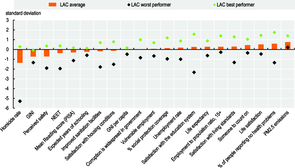
Note: This figure is based on a cross-country bivariate regression of each well-being indicator against GDP per capita across all countries in the world with population above 1 million. The coefficient of this regression, alongside the GDP per capita of each country and region, allows computing the expected value that each well-being variable should attain given the GDP per capita of the region or country. Actual values for each variable are compared to expected ones with the difference standardised by the standard deviation of the indicator. In this way, the figure highlights areas of well-being where the region (or individual countries within it) is performing better or worse. GNI is used as a proxy for household income. Mean reading score from the Programme for International Student Assessment is used as a proxy of quality of education. LAC countries include Argentina, Bolivia, Brazil, Chile, Colombia, Costa Rica, Cuba, Dominican Republic, Ecuador, El Salvador, Guatemala, Haiti, Honduras, Jamaica, Mexico, Nicaragua, Panama, Paraguay, Peru, Trinidad and Tobago, Uruguay and Venezuela. NEET=Not in education, employment or training. GINI coefficient measures the inequality of levels of income.
Source: Own calculations based on OECD (2015); Gallup (2017); UNDP (2017); UNESCO (2018); UNODC (2018); World Bank (2018).
There are also significant cross-country differences within the LAC region for each well-being dimension. Gaps between worst and best regional performer values are much larger in the share of people with no health problems, satisfaction with the education system and affected by homicides.
Heterogeneity within income-groups in Latin America and the Caribbean
LAC countries with higher income per capita do not always perform better in terms of development outcomes than countries in the region with lower income per capita. Development challenges persist even when countries cross a given income level. Development performance tends to be higher among LAC countries with the highest income per capita. However, high income per capita alone does not guarantee high performance across all development indicators.
Using an average income measure, such as GDP or gross national income (GNI) per capita, can hide strong disparities across countries in different essential aspects of people’s lives. At the international level, countries are usually classified in four income groups: low-income, lower middle-income, upper middle-income and high-income according to their level of GNI per capita. The OECD Development Assistance Committee list of official development assistance (ODA) recipients is defined through the GNI per capita.
Most LAC countries are upper middle-income, including Brazil, Colombia, Costa Rica, Dominican Republic, Ecuador, Jamaica, Mexico and Peru. Other countries, such as Argentina, Chile, Panama, Trinidad and Tobago, and Uruguay, are classified as high-income countries, while only Haiti is a low-income country (Figure 2.2). Although LAC countries in each group share common characteristics, belonging to one of these groups does not necessarily entail similar outcomes across the multiple dimensions of development.
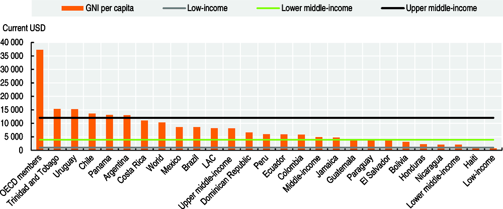
Note: Only countries with more than 1 million population were included. GNI data for Aruba, Cuba, Curacao, St. Martin (French part), Sint. Marteen (Dutch part), Turks and Caicos Islands, Venezuela, British Virgin Islands and Virgin Islands (US) are missing. Antigua and Barbuda, Bahamas, Barbados, Belize, Dominica, Grenada, Guyana, St. Kitts and Nevis, St. Lucia, St. Vincent and the Grenadines and Suriname were not included because their population is below 1 million inhabitants. See Chapter 6 for an analysis on the Caribbean small states.
Source: World Bank (2018), World Development Indicators.
Overall, LAC countries perform poorly in selected development outcomes compared to their worldwide income category peers. This is particularly evident for higher-income countries. For instance, high-income countries in LAC lag behind in terms of homicide rates, inequality, vulnerable employment and satisfaction with healthcare compared to high-income countries worldwide (Figure 2.3, Panels A, B, C and D). At the same time, on average, all three LAC income groups have higher homicide rates than their corresponding worldwide income groups (Figure 2.3, Panel A).
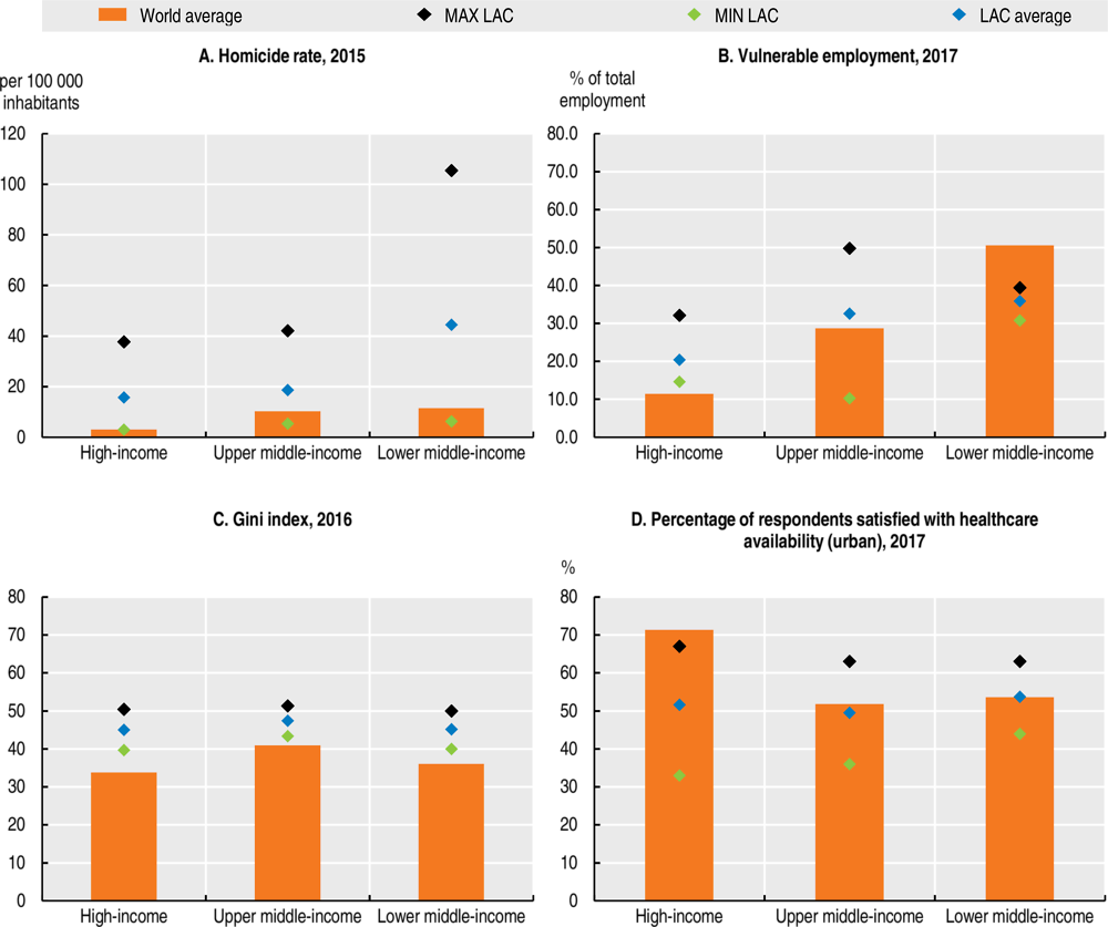
Note: Simple averages are used both for LAC and world averages. LAC lower middle-income countries include Bolivia, El Salvador, Honduras and Nicaragua. LAC upper middle-income countries include Belize, Brazil, Colombia, Costa Rica, Cuba, Ecuador, Grenada, Guatemala, Guyana, Jamaica, Mexico, Paraguay and Peru. LAC high-income countries include Argentina, Bahamas, Barbados, Chile, Panama, Puerto Rico, Trinidad and Tobago and Uruguay.
Source: Own calculations based on World Bank (2018), UNODC (2018) and Gallup (2017).
Among the LAC countries with available data, development outcomes are mixed across income groups. High-income countries do not always perform better than middle-income or lower-income countries. In fact, with respect to income inequality and satisfaction with healthcare, lower-income countries perform better than upper middle-income countries (Figure 2.3, Panels B and D).
The mixed development outcomes occur partially because LAC countries’ individual performance across selected indicators varies considerably among countries belonging to the same income group. For instance, the homicide rate of El Salvador (105 deaths per 100 000 inhabitants) is 17 times the homicide rate of Bolivia (6 deaths per 100 000 inhabitants), while both countries are lower middle-income economies (Figure 2.3, Panel A). Similarly, vulnerable employment is 40.6 percentage points higher between the best performing and worst performing upper middle-income country in LAC (49.7% in Peru and 10.3% in Cuba) (Figure 2.3, Panel C). The share of people satisfied with the healthcare system varies considerably among LAC high-income countries, from 67% in Uruguay to 33% in Chile (Figure 2.3, Panel D).
Heterogeneity is so large among income groups that in several development outcomes lower-income countries in LAC perform better than middle-income and even high-income countries. For instance, Trinidad and Tobago, and Uruguay, both high-income countries, present homicide rates greater than Bolivia, the best performer of the lower middle-income group, as well as for the average for all three income groups (Figure 2.3, Panel A). Similarly, inequality in Panama, the worst-performing country of the high-income group, is higher than in Mexico and El Salvador, the best-performing countries of the upper middle-income group and lower middle-income group, respectively. Meanwhile, the share of people satisfied with their healthcare system in Nicaragua (63%), the best performer of the lower middle-income group, is greater than in Brazil (36%) and Chile (33%), the worst-performing countries of the upper middle-income and high-income groups, respectively.
All in all, the income level group for a country does not provide a full picture of its performance across all development dimensions nor its challenges.
Subnational heterogeneity in development outcomes
Subnational regions and cities in LAC display considerable differences in well-being outcomes relative to national averages. National averages generally hide large diversity across subnational regions in all continents, but the pattern is especially pronounced in LAC (OECD, 2016a). The need for a regional lens when considering well-being outcomes is key to better understanding differences in the region and in better designing public policies to address them.
Subnational differences in LAC characterise all well-being outcomes and are evident when considering GDP per capita. LAC’s territorial disparities in GDP per capita are striking, and much larger than in OECD member countries. Subnational differences in GDP per capita (as measured by the Gini coefficient in average GDP per capita across regions) in OECD member countries is around 16%. However, in some LAC countries such as Brazil, Chile, Colombia, Mexico and Peru, subnational differences are close to or higher than 30% (OECD, 2016a). Moreover, GDP per capita does not truly reflect average differences in GNI since regions that rely on oil and other commodities can have both high GDP and low average national income.
Subnational regions with high income per capita coexist with lower income per capita regions in most LAC countries (Figure 2.4). This is particularly evident in Colombia, Mexico and Peru where high-income subnational regions coexist with others with upper and lower middle-income (Figure 2.4, Panels C and E). When states and provinces within each country are evaluated based on a proxy of GNI1, the conventional ODA graduation criterion, their disparities can be measured as “years to graduation”. In Mexico, for instance, Ciudad de Mexico became high-income more than 13 years ago when it achieved a GNI per capita of USD 12 056; while Chiapas will achieve high-income status in 60 years assuming the growth rate of its GNI per capita remains constant. Likewise, Chile became a high-income country in 2013, but half of its regions, where one-third of the country’s population live, still have a GNI per capita below the graduation threshold of USD 12 056. Similarly, the capital cities of Brazil, Colombia and Peru have a per capita GNI of more than twice that of half the provinces of their country.
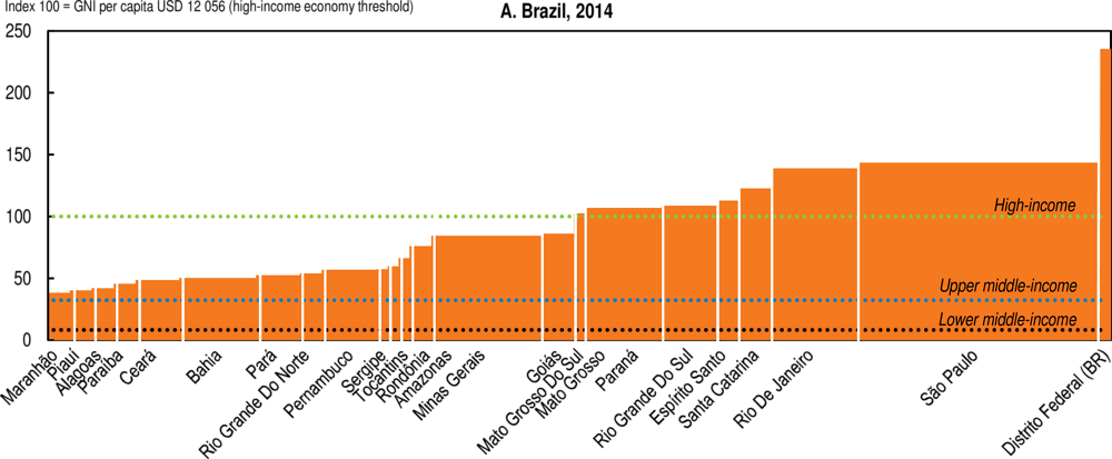
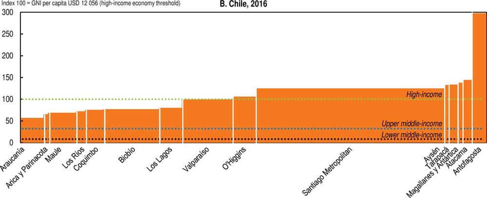
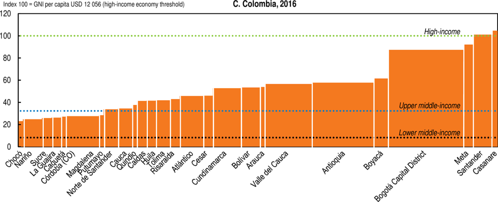
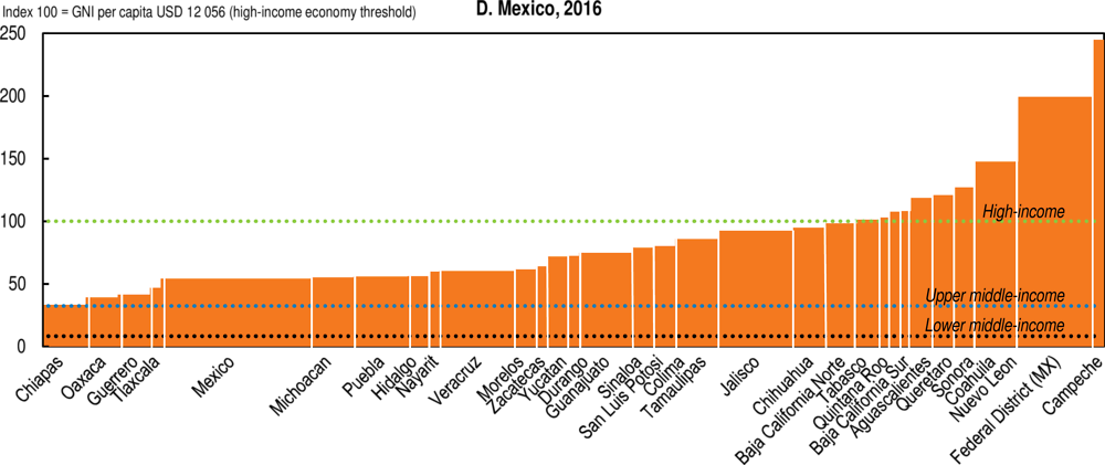
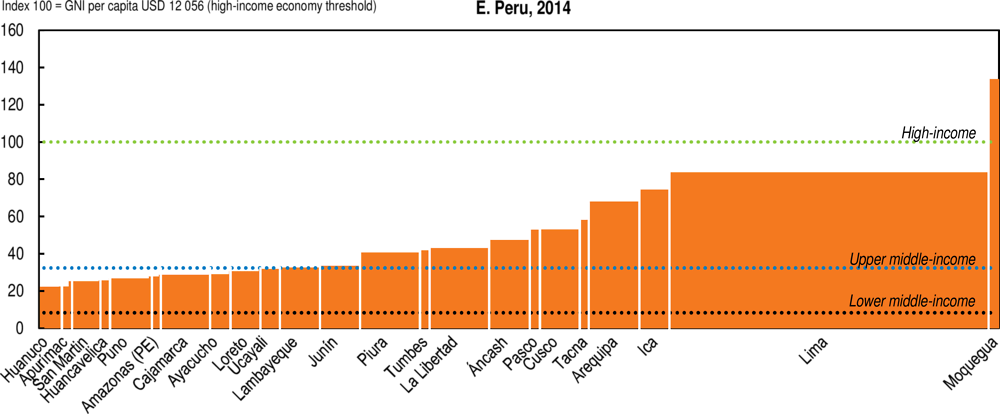
Note: Thresholds are the following: high-income economies (those with a GNI per capita of USD 12 056 or more) index = 100. Upper middle-income economies (those with a GNI per capita of USD 3 896 or more) index = 32.3. Lower-middle-income (those with a GNI per capita of USD 996 or more) index = 8.3. World Bank country classification for 2018-19. Regional GNIs were based on a three-step calculation that assumes GDP and GNI follow the same regional distribution. First, the difference between the national GDP and GNI of each country is calculated. Second, each region’s share of this difference is calculated based on its share of national GDP. Third, each region’s share of the difference between national GDP and GNI is subtracted from its regional GDP. Regions with a population 1% of the national population were not included. These include Vaupes, Guainia, Vichada, Guavarie, Amazonas and San Andres in Colombia; Madre de Dios in Peru; and Acre, Amapa and Roraima in Brazil.
Source: Own calculations based on OECD (2018e).
There are also large gaps within LAC countries with respect to other well-being measures. Well-being inequality in LAC countries is closely linked to where people live and work. The “urban advantage” remains strong when looking at other development measures, especially in high-income countries such as Argentina and Chile. Large LAC cities, especially capitals, have better education, employment and health, and lower poverty outcomes than most small cities and rural areas. Many more children in rural areas die before the age of 1 year due to lack of access to basic healthcare than in urban areas in LAC. For example, infant mortality in Boca del Toro, a rural province in Panama with a share of 1% of the country’s GDP, is more than twice that of Panama City, which is responsible for 75% of the country’s output. Likewise, on average, youth in states and provinces with large rural areas leave school earlier than those in regions with large urban areas. Conversely, crime and violence are higher in the regions with larger cities.
Territorial disparities are largest for poverty and informality rates. Colombia and Mexico have the largest regional differences in national income poverty. In Mexico, only 14.2% of the population in Nuevo Leon live under the national income poverty line; while 77.1% of the population do so in Chiapas (INEGI, 2018). Likewise, in Colombia, 12.4% of the population of Bogota live below the poverty line, while the poverty rate of Chocó is 58.7%. Regional gaps in terms of informality are also wide across most LAC countries analysed in this section, ranging from 12.6 percentage points in Costa Rica to 45.1 percentage points in Mexico. Most countries have a gap of around 35 percentage points (Figure 2.5).
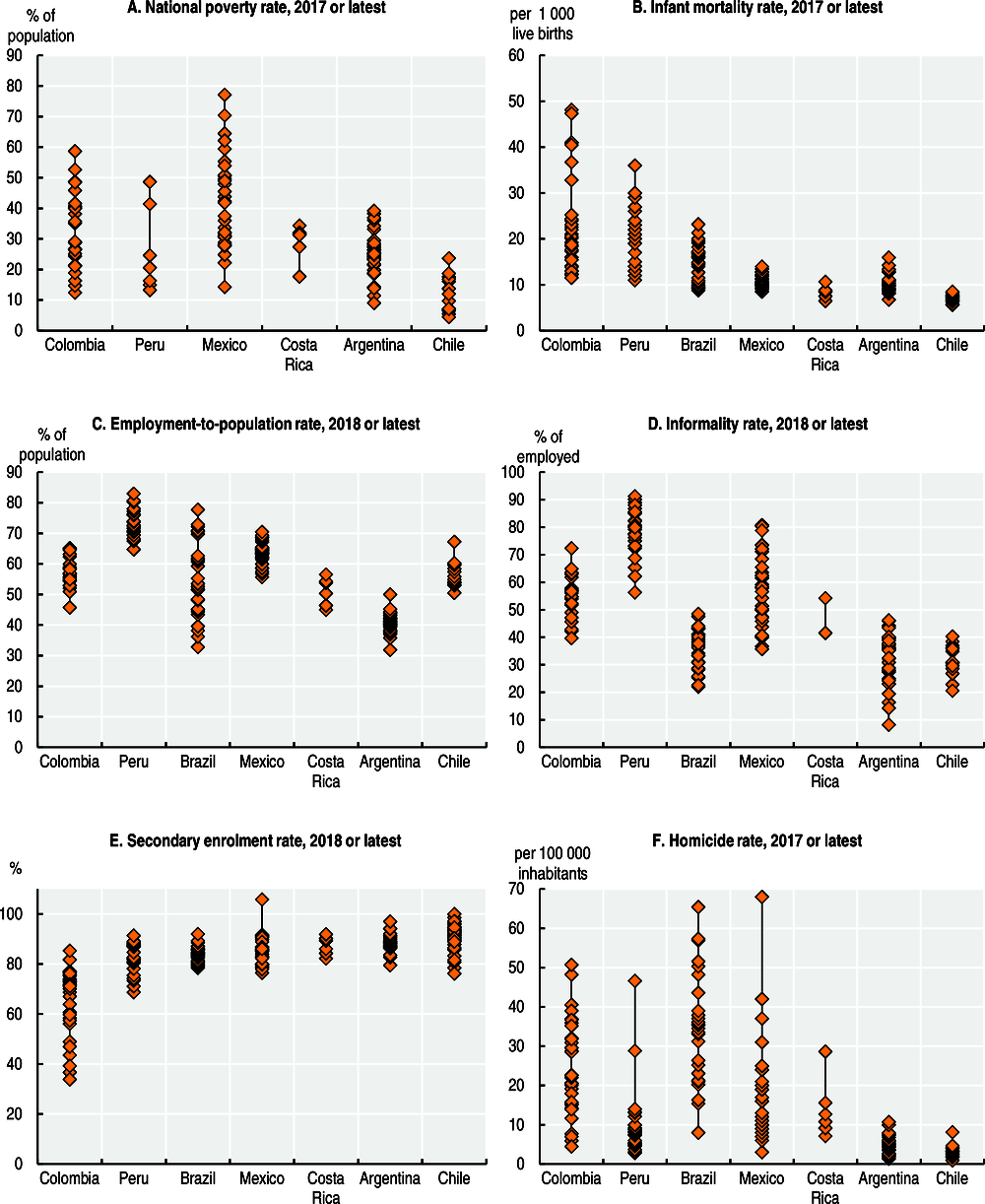
Note: Each marker represents a province, state or region within a country. Countries ordered by level of GDP per capita. For the employment and informality indicators, working-age population refers to people aged 14 or older in Argentina and Peru, 15 or older in Costa Rica and Chile, 16 or older in Brazil, 12 or older in urban areas of Colombia and 10 or older in rural areas of Colombia. The informality figures for Brazil are based on authors’ calculations with data from IBGE (2018): they include independent workers not registered in National Registry of Legal Entities (CNPJ-Cadastro Nacional da Pessoa Jurídica) and dependent workers without a signed work contract.
Source: Centre for the Study and Analysis of Crimes in Chile (2018), CONAPO (2018), CONEVAL (2016), DANE (2018a, 2018b, 2018c), IBGE (2017, 2016, 2015), IGARAPE (2018a, 2018b, 2018c), INDEC (2018, 2017a, 2017b, 2017c), INE (2017, 2015), INEC (2016, 2017a, 2017b, 2017c), INEGI (2017, 2015), INEI (2018a, 2018b, 2015a, 2015b), Ministry of ICT of Colombia (2018), Ministry of Labour and Employment Promotion of Peru (2015), Ministry of Social Development of Chile (2017), OECD (2016b), RIMISP (2018).
Territorial disparities in infant mortality are also wide. For example, in Colombia, the infant mortality of Vichada is almost three times that of Antioquia (DANE, 2018a); in Peru, the infant mortality of Tumbes is over three times higher than that observed in Puno (INEI, 2015a).
In terms of homicide rate, territorial differences vary between countries in LAC. Brazil, Colombia, Mexico and Peru have large gaps in homicide across regions (Figure 2.5). These gaps are much lower in Costa Rica and almost non-existent in Argentina and Chile (Figure 2.5).
The benefits of education are also spread unevenly across regions. Territorial-related differences are less marked than for other development outcomes in most countries except Colombia. Secondary enrolment rates are 10 percentage points higher in the region with the highest share of youth enrolled in secondary education than in the one with the lowest share in Brazil and Costa Rica. The gap in Colombia exceeds 50 percentage points (Figure 2.5).
Addressing regional disparities should be a key element of any development strategy in LAC. The factors that most influence peoples’ well-being are local, such as employment, access to health services and education, and security. Policy responses must also be locally targeted. Policies that take better account of regional problems and needs may have a greater impact in terms of improving well-being for the country as a whole by tackling the sources of inequality more directly. But to target policies effectively, governments need the tools to fully understand local conditions and the expectations of their citizens (OECD, 2016a).
Large cross-country differences in domestic resource mobilisation
Despite moving to high-income or upper middle status, some LAC countries are still unable to meet their financial needs due to low tax revenues. Country groupings based on GDP per capita hide disparities in countries’ abilities to mobilise domestic resources to face development challenges. A high level of GDP per capita is not always associated with greater tax capacity.
LAC countries show a mixed performance in terms of their tax capacities; differences are only weakly related to their GDP per capita level. For instance, in all high-income economies in LAC, the level of taxes mobilised to fund development is below the world average of high-income countries (Figure 2.6). Similarly, several LAC high- or middle-income economies might be unable to meet their future financial needs given their tax-to-GDP ratios are similar to or below those of lower middle-income economies (see Chapter 4 for an analysis on domestic resource mobilisation).
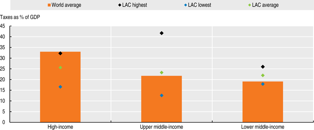
Note: Bars represent the world average across the 80 countries covered in the OECD Global Revenue Statistics (25 in LAC, 18 in Africa, 35 in the OECD and 4 in Asia). In LAC, high-income economies include Argentina, Bahamas, Barbados, Chile, Panama, Trinidad and Tobago, and Uruguay. Lower middle-income economies include Bolivia, El Salvador, Honduras and Nicaragua, and upper middle-income economies include Belize, Brazil, Colombia, Costa Rica, Cuba, Dominican Republic, Ecuador, Guatemala, Jamaica, Mexico, Paraguay, Peru and Venezuela. Countries are classified by income groups according to World Bank methodology. The flat line represents the simple average of LAC economies depending on their income group (https://datahelpdesk.worldbank.org/knowledgebase/articles/906519-world-bank-country-and-lending-groups).
Source: Own calculations based on OECD (2018c).
copy the linklink copied! Links between GDP per capita and well-being outcomes weaken when moving up the income ladder
In the LAC region, the relationship between levels of GDP per capita and well-being outcomes is not uniform across the income ladder. In other words, high-income countries may feature worse development outcomes than upper middle-income countries. For their part, upper middle-income countries may confront development challenges as serious as those encountered by low-income ones. A similar phenomenon emerges when comparing changes in GDP per capita to changes in well-being outcomes. Availability of comparable time-series for key well-being outcomes for LAC countries is even more limited than for recent estimates. However, analysis in this section shows that trends in real GDP per capita do not fully reflect changes in other dimensions of well-being such as life expectancy, education, security or income inequality.
The analysis rests on estimates by a group of economic historians charting long-term developments in GDP and in a range of well-being outcomes across the world (van Zanden et al., 2014). Based on these estimates, this section looks at the relationship between a composite well-being measure and the seven individual series included in this composite, on one side, and GDP per capita on the other over time. While historical research must contend with many data limitations, this section aims to investigate the strength of the association between GDP per capita and well-being, as well as to understand changes in this association as countries’ GDP grows.
Although the value of considering multiple indicators of well-being is clear, a composite measure can provide valuable information about well-being when all the indicators are considered at the same time. While policies require looking at each individual variable, a composite allows assessment of how countries compensate for a bad performance in one aspect of well-being with a good performance in another.
Aggregating multiple indicators into one composite is not without problems. Trade-offs exist in every composite indicator and all approaches to constructing a composite indicator have advantages and disadvantages (Ravallion, 2011). The composite indicator used in this section (Box 2.1) is constructed through a latent variable model similar to that used in How Was Life? (van Zanden et al., 2014). This approach allows dealing with missing data and accounting for the uncertainty that arises. Yet this inevitably comes at a price in terms of transparency (van Zanden et al., 2014).
This section uses historical estimates on six well-being dimensions to construct a single well-being composite indicator. The indicator mirrors the one included by the OECD in its well-being report How’s Life? (OECD, 2011), and draws on the best sources and expertise available for historical perspectives in this field. Although it was constructed using variables available for a large set of countries and long-term trends, historical data on well-being are limited and significant gaps remain.
The six indicators considered aim to provide information on how the benefits from economic growth are spread across society. They pertain to real wages of unskilled workers in the building industry, which provide information on the living standards of wage earners; life expectancy at birth, a standard measure of population health; average population height, a measure mainly affected by nutrition during the first years of life; average years of schooling, a measure of the quantity of education; a (composite) measure of political institutions, i.e. the Polity2 Index of autocracy-democracy; countries’ homicide rates, a measure of personal security; and the Gini coefficient on gross household per capita income, a measure of income inequality.
The composite measure provides a parsimonious view of the evolution of well-being in each country. To construct this composite indicator, a latent variable (factor) model was used as in van Zanden et al. (2014) and Rijpma (2017). In this model, indicators are assumed to be correlated with each other because of their correlation with a latent variable. For this assumption to hold, a single concept of well-being linked to the observable indicators has to be plausible at the cross-country level. Before running the model, individual indicators were standardised so that the mean and standard deviations for the 1900-2010 period and all countries are zero and one respectively. Following advice in Ravallion (2011) and Chakravarty (2003), no further transformations were performed on the data.
Specifically, this section uses the composite measure by Rijpma (2017) since it does not include GDP per capita. The analysis aims to perform a simple linear rolling panel fixed effect regression with real GDP per capita (USD 2011) as the independent variable and the composite well-being indicator as the dependent variable. Hence, a composite indicator of well-being that included GDP per capita as one of its components would have implied an endogeneity bias.
The data used in the analysis cover 183 countries between 1900 and 2010. Owing to particularities of the data and missing values along the historical evolution, ten-year averages are used. Data were standardised using the formula:
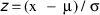
where μ is the mean and σ the standard deviation.
Regional averages are constructed for comparison. The LAC average includes all countries in the Americas except the United States and Canada. The Southeast Asia average includes the People’s Republic of China (hereafter “China”); Hong Kong, China; Japan; Korea and the rest of Asia excluding the countries to the west of Afghanistan. OECD covers all member countries.
GDP per capita is strongly associated with the composite well-being measure for countries with low level of GDP per capita. Up to a level of around USD 2 000 (2011 PPP), every additional standard deviation of GDP per capita increases the composite well-being measure by around eight standard deviations (Figure 2.7).
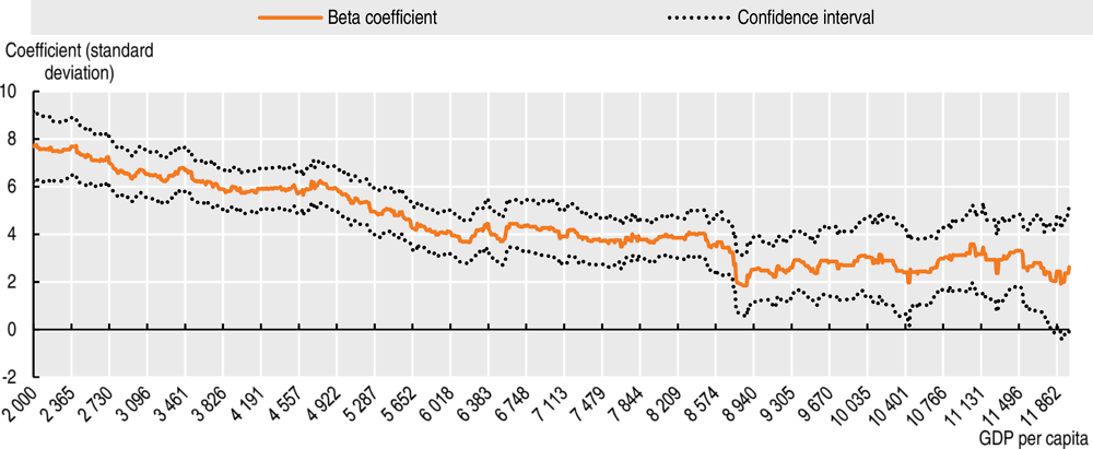
Note: Beta coefficients of a rolling fixed-effects panel regression across the income ladder (see Box 2.2).
Source: Own calculations based on https://www.clio-infra.eu/ and Rijpma (2017).
GDP per capita and well-being outcomes gradually delink as countries become richer in terms of GDP per capita. The association between GDP per capita and the composite well-being measure (as well as with the individual well-being variables that make up this composite) become weaker when moving further up the income ladder. In other words, the link between GDP per capita and well-being weakens among richer countries. In fact, the association between the composite well-being measure and GDP per capita is more than twice as large for low-income countries than for upper middle-income countries, and almost three times stronger than for high-income economies. For upper middle-income countries, those with a GDP per capita of around USD 7 250 (2011 PPP), an increase of one standard deviation in GDP per capita increases the composite well-being measure by only four standard deviations. At income levels of USD 11 750 (2011 PPP) and more, on average, an increase of one standard deviation in GDP per capita increases the composite well-being measure by only three standard deviations (Box 2.2).
This exercise assesses the relationship between the well-being composite and GDP per capita across the income ladder, as well as the residual of this regression and individual well-being indicators.
In a first step, a rolling panel fixed-effect regression is performed across the income ladder (with no time fixed effect). The independent variable is GDP per capita (at USD 2011 PPP) and the dependent variable is the composite well-being indicator (see Box 2.1 for explanation on the construction of the variable):
 (1)
(1)
The rolling regression is done based on GDP per capita with a window of USD 3 000 (2011 PPP) that evolves by USD 10 (2011 PPP).1
Additionally, the same regression is performed using as dependent variables each of the indicators from the well-being composite (i.e. real wages, income inequality, life expectancy, height, years of education and homicide rates). It regresses them against GDP per capita as independent variable in a rolling panel fixed-effect regression across the income ladder.
In a second step, this exercise uses the residuals  from the regression as dependent variable to run a rolling panel country-fixed effects regression against the different well-being dimensions shown in Table 2.1 (with a similarly sized window and evolution). The results of this second exercise are presented in Annex 2.A1. The model assumes that well-being can be characterised according to the following equation:
 (2)
(2)
Overall, this exercise aims to find which dimensions of welfare explain people’s well-being given that GDP per capita does not fully translate into quality of life.
The results should be taken with caution as this methodology is not without its limits. First, it assumes a linear relationship across the different well-being dimensions and GDP per capita. Second, as the regression does not control for time, coefficients may capture differences across countries rather than levels of development. Third, the data are from 1900 to 2010; although considerable effort has been taken to make data comparable, quality fluctuates by country and time (van Zanden et al., 2014).
← 1. The size of the window of the rolling regression was 3 000. Both the size of the window and its evolution were chosen based on data availability. Other windows of GDP per capita of 1 000, 2 000 and 15 000 were also tested with similar results.
The same delinking between GDP per capita and the composite well-being measure also holds when looking at individual measures included in the composite. This pattern is most pronounced for life expectancy, educational attainment and real wages (Figure 2.8). Although at a slower pace, homicide rate, income inequality and height delink from GDP per capita as countries become wealthier. This is especially the case when countries surpass the upper middle-income threshold of GDP per capita of USD 7 250, 2011 PPP.
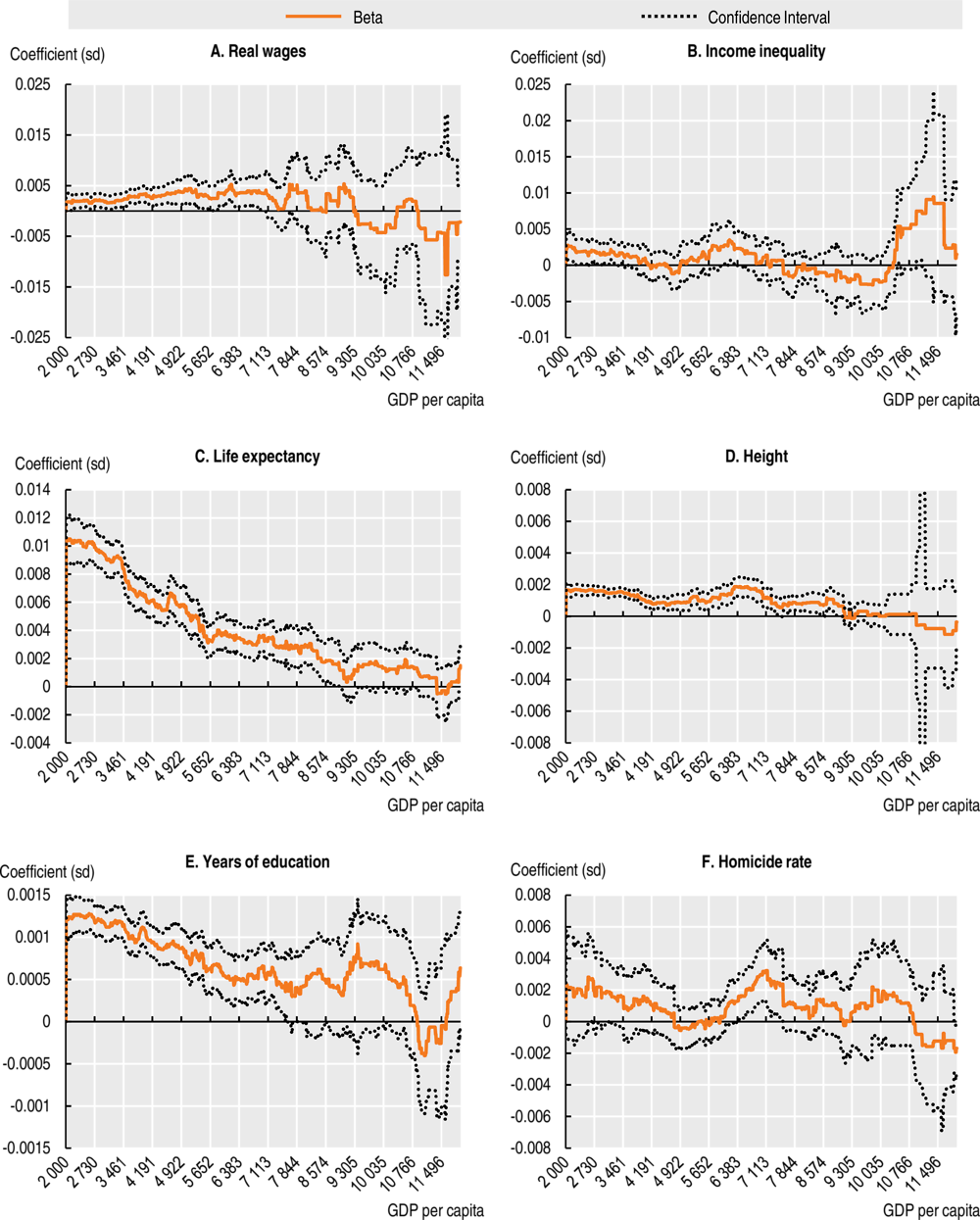
Note: Beta coefficients of a rolling fixed-effects panel regression across the income ladder (see Box 2.2).
Source: Own calculations based on www.clio-infra.eu/ and Rijpma (2017).
As LAC economies grow, several development dimensions other than GDP per capita become more important in improving people’s lives. As countries climb the income ladder, the association between life expectancy, education, personal security and democratic stability, and the residual of the regression between GDP per capita and the well-being composite indicator (the error term in the previous analysis), gains strength and significance. This relationship is most evident in the case of life expectancy (See Annex 2.A1.).
copy the linklink copied! Actual versus expected well-being outcomes in Latin America and the Caribbean over time
The relationship between various dimensions of well-being and GDP per capita has also changed over time. At the global level, there was no additional well-being accrued beyond that explained by higher per capita GDP for most well-being indicators in the 19th century. This changed, however, in the 20th century as some well-being indicators began delinking from GDP per capita (OECD, 2018a). While the LAC region had higher GDP per capita than several other world regions in the past century, it did not always achieve better well-being outcomes.
This section compares the LAC average performance for seven well-being variables to the one expected given its GDP per capita from 1950 to 2010 (for methodology see Box 2.3). Evidence shows that GDP per capita has not always been a good predictor of the various dimensions of well-being in LAC. While some well-being outcomes increased more rapidly than implied by GDP growth alone, others increased at a slower pace.
To assess the relationship between the different dimensions of well-being and GDP per capita, a simple linear regression model (OLS) has been run. The dependent variable is a single well-being dimension (see Box 2.1 for list) and the independent variable is the logarithm of GDP per capita (USD 2011). The different well-being dimensions can be characterised according to the following equation:

The coefficient  is used to obtain a predicted or expected level for all well-being indicators according to the level of GDP per capita. Finally, ten-year averages are computed to present the results over time.
The analysis is based on a panel dataset composed of 183 countries worldwide, including 22 LAC countries from 1900 to 2010. The final dataset has 2 552 observations. The analysis is based on Clio Infra (database), except for GDP per capita (2011 USD), which is sourced from the Maddison dataset.
Real wages in LAC are lower than those expected based on GDP per capita. Although GDP per capita is strongly correlated with real wages, the difference between the expected and the observed levels are large and statistically significant for most of the period covered by available data (from 1960 up to 2005, the difference is at least at the 10% level). Since 1950, the region’s real wages have consistently lagged behind the level observed in countries with similar levels of GDP per capita (Figure 2.9, Panel A).
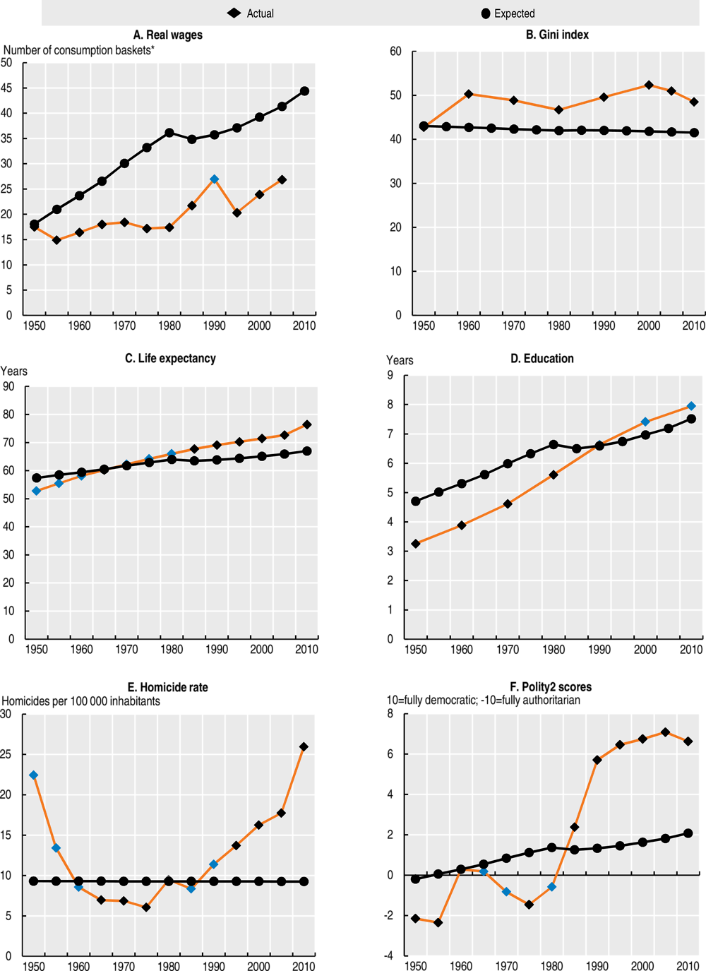
Note: * Real wages are measured as the number of consumption baskets purchased with the real wages of a male unskilled worker in the building industry.
Expected values are calculated with a panel dataset composed of 183 countries worldwide from 1900 to 2010. Actual values not statistically significant, at least at the 10% level, were signalled in blue. In the case of the Gini coefficient, the series was expanded for 2005 and 2010 using growth rates from the CEPALSTAT Gini series for LAC. The LAC average includes all countries in the Americas except Canada and the United States.
Source: Own calculations based on www.clio-infra.eu/ and CEPALSTAT.
Informality is one of the main obstacles to higher wages and to a more inclusive labour market. A large share of the working-age population encounters labour-market difficulties due to insufficient work-related skills, lack of quality jobs and territorial disparities. Improving job quality, reducing informality and increasing employment levels – especially for women and youth – are key challenges for improving material conditions and equity (OECD/CAF/ECLAC, 2016).
Income inequality has been higher in LAC than expected based on GDP per capita. Although income inequality has declined since the 2000s in most LAC countries, it has slowly increased since the 1980s at a regional level. Both current and expected levels of income inequality are only weakly related to countries’ GDP per capita. The differences between the two are statistically significant since 1960 for every period where data are available (at least at the 10% level).
Income inequality is the dimension of well-being, from the ones analysed in this section, that best illustrated the problem of using GDP per capita as a sufficient condition for development. GDP growth is much needed for countries to improve people’s well-being, but is not enough (Figure 2.9, Panel B). Lowering income inequalities in the region requires more than higher GDP.
Life expectancy in LAC tracked closely its predicted value between the 1950s and 1980s. Since the 1980s, the region’s life expectancy delinked from GDP per capita and exceeded the level expected. A statistically significant gap remained between the two (at least at the 10% level) (Figure 2.9, Panel C).
LAC’s educational attainment exceeds the level expected given the region’s GDP per capita. Average years of education of the population of LAC were below the levels expected between 1950 and 1985. Since the 1990s, LAC’s performance in education exceeded expectations as a result of policies to expand education coverage, especially at primary level (Figure 2.9, Panel D).
Yet education quality remains a pressing concern throughout the region. More than half of 15-year-old Latin Americans enrolled in school do not have basic proficiency in reading, mathematics and science (OECD, 2016b). Fewer than 1% of LAC students perform at the highest levels of proficiency in mathematics, reading or science. Lack of proficiency in these areas is an obstacle to developing more specific skills later in life and may hamper innovation and entrepreneurship. This is a major challenge for LAC countries as they try to transition into knowledge-based economies where citizens need to innovate, adapt and leverage advanced human capital (OECD/CAF/ECLAC, 2016).
Personal security in LAC is much worse than expected based on economic performance. Homicide rates fell significantly between the 1960s and the 1980s, but increased sharply from 1985 onwards. The rates far exceeded predicted levels, with a statistically significant difference since 1995 (at least at the 10% level) (Figure 2.9, Panel E).
Democratic stability has been strengthening in the region in recent decades. Since the beginning of the 20th century, democratic stability in LAC has been a winding path. It was hindered sizably between 1960 and 1970 when most LAC countries were ruled by military dictatorships. However, since the 1980s, when the region experienced the third wave of democratisation (Huntington, 1991), democratic stability has been strengthening, surpassing that of other countries with similar levels of GDP per capita. Since 1990, the difference between expected and observed is statistically significant (at least at the 10% level) (Figure 2.9, Panel F).
Over the last decades, LAC’s GDP performance has not rendered into the better real wages, lower inequality and greater security expected. Income thresholds ignore the complex nature of development and the diversity and heterogeneity of countries in transition. Development must be conceived as a multifaceted process consistent with facing the structural challenges of a particular country rather than as a one-size-fits-all approach based on grouping the countries according to their income levels.
copy the linklink copied! Multi-dimensional approach to measure development: Going beyond GDP
A broader concept of development requires a different approach to measurement. Moving beyond GDP metrics as the sole indicator of success requires measures for a broad range of development outcomes. This includes using data on how well-being outcomes are distributed across a population and local areas, as well as on sustainability.
To go beyond GDP, countries should focus more on people’s well-being and societal progress. They should look not only at the functioning of the economic system, but also at the diverse experiences and at living conditions of people. These kinds of measurements are key to understanding what drives well-being of people and nations, and what is needed to achieve greater progress for all.
To assess development outcomes beyond GDP, LAC countries need first to identify the dimensions of life that matter most for people and the resources needed to ensure sustainability. Concurrently, LAC countries should operationalise all these dimensions through a set of indicators, as well as collect data on country averages and both vertical and horizontal inequalities.
Beyond statistical capacity and co-ordination of national initiatives, developing indicators that can capture key concerns for LAC requires building consensus around the most relevant issues and challenges confronted by national governments in the region. To be sustainable and to provide the basis for policy dialogue and co-operation within the region, a wide range of stakeholders must take part in the process of consensus-building.
After having identified the most relevant development outcomes for the region, a significant data challenge remains: most LAC countries lack comparable data for many key well-being domains shaping people’s lives. These domains range from households’ material conditions to more qualitative aspects such as job quality, trust in other people and in institutions, people’s self-reports of their own lives, social connections or pressures on natural resources. Such data challenges are all the more important as monitoring development outcomes to inform policy requires data that look beyond averages. Specifically, data should consider inequalities in all life dimensions and assess the conditions of different population groups (e.g. by gender, age, race and ethnicity, place or living). Co-ordinated efforts are therefore needed to reach agreement on a well-being framework for the region, to develop the capacity needed to fill data gaps, and to improve comparability and disaggregation of selected measures.
In response to the challenge, the European Union, the OECD and the UN Economic Commission for Latin America and the Caribbean are launching a project to develop improved metrics of well-being and multi-dimensional development for the region. The project, “New metrics for development: A well-being approach to improving people’s lives in Latin America”, is part of a broader Regional Facility for Development in Transition in Latin America and the Caribbean.
Over three years (2018-21), the project has three aims:
-
to develop a well-being framework adapted to the realities and priorities of Latin American and Caribbean countries
-
to populate this framework with higher quality and more granular data than those available and used in this chapter, to be developed in co-operation with national statistical offices in the region
-
to support policy makers in identifying development priorities and designing policies and programmes to achieve them, based on the metrics developed in the context of the project.
copy the linklink copied! Conclusions
Despite considerable progress in the past century, GDP growth has not always translated to similar well-being gains for Latin American people. As LAC countries moved up the income ladder, violence and income inequality grew. At the same time, informality has become a persistent problem. Real wages have increased at a slower pace than in other countries in the world with similar income per capita. Though school enrolment has increased, access to higher education and quality secondary school are still limited to a privileged group. While Latin Americans live, on average, almost as long as citizens of OECD countries, they face more health problems. In sum, economic gains have improved certain areas of development, but not other longstanding challenges. They have also raised new problems (OECD, 2018a).
Policy makers need to re-conceptualise development and to rethink both domestic policies and international co-operation to “leave no-one behind” and fulfil the goals of the 2030 Agenda (see Chapters 4 and 5). In this context, it is essential to acknowledge the heterogeneity across countries in terms of their development challenges, which are often independent of their income. This is particularly important for LAC countries that are transitioning to higher-income levels, but still lack capacity to compete and narrow their economic and social gaps relative to more advanced developed countries (Barcena, Manservisi and Pezzini, 2017).
Income per capita can provide a ballpark idea of the development challenges confronting each country in the region. However, it fails to draw the detailed print that policy makers need as a roadmap to achieve sustainable development. Indeed, the relationship between GDP per capita and well-being varies across the income ladder. Furthermore, as economies grow, other dimensions of welfare beyond GDP take over as co-determinants of well-being.
Looking at development through a multi-dimensional lens serves as a good compass to design, implement, monitor and evaluate policies to improve people’s lives. The evidence in this chapter confirms that material living conditions, and especially income, matter. But it also shows that income per capita is not the only feature shaping people’s lives and well-being. Quality jobs, health, education, democracy, personal security and inequality are important as well. And they are especially important for well-being as countries grow.
Flawed measurement tools will distort policy making (Stiglitz, Sen and Fitoussi, 2009). LAC countries should invest in better data collection to measure and monitor those well-being dimensions that are most important for the region across their territory and population groups. In this process, consultation with different stakeholders is crucial to build a shared understanding of what well-being dimensions have been acclaimed to matter the most. Efforts should be made to produce accessible, timely and disaggregated data. This is a remarkable challenge for all countries, and especially so for those in transition. Achieving these goals through building national statistical capacity is critical to establish where each country stands, to prepare long-term development plans and to monitor progress along the way.
As economies grow in terms of GDP per capita, other dimensions of welfare, such as life expectancy, education, personal security and democratic stability take over as co-determinants of well-being.
This exercise is based on the empirical analysis described in Box 2.2 that uses the following regression:
 (1)
(1)
This exercise uses the residuals  from the regression as dependent variable to run a rolling panel country fixed effects against the different well-being dimensions shown in Table 2.1 (with a similarly sized window and evolution). The model assumes that well-being can be characterised according to the following equation:
 (2)
(2)
Overall, this exercise aims to find which dimensions of welfare explain people’s well-being given that GDP per capita does not fully translate into quality of life.
Results show that the relationship between the portion of well-being that cannot be explained by GDP per capita (the error term in the previous analysis) and the life expectancy of countries strengthens at higher levels of income (Annex Figure 2.A1.1, Panel A). In fact, at low level of income, an additional standard deviation in life expectancy is to increase by 0.4 standard deviation the portion of well-being unexplained by GDP per capita. At higher level of income, this impact increases up to one standard.
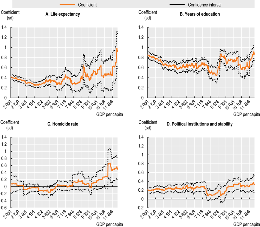
Note: Beta coefficients of a rolling fixed-effects panel regression across the income ladder (see Box 2.2).
Source: Own calculations based on https://www.clio-infra.eu/ and Rijpma 2017.
Additionally, education stands out as another key dimension of well-being. At all income levels, education plays an important role in explaining the part of well-being that GDP per capita fails to do. Having basic notions of reading or mathematics makes everyday life easier for transactions, for example. As well, knowledge can be an intrinsic pleasure for individuals (OECD, 2011). Besides, education can foster economic development (Romer, 1990) or increase political stability (Alesina and Perotti, 1996), which indirectly affects well-being. Although the results are relatively constant across country levels of GDP per capita, the association between years of education and well-being shows a slight increase around USD 8 500 (2011 PPP) (Annex Figure 2.A1.1, Panel B).
Personal security and democratic stability are also positively associated with higher levels of well-being. As in the case of life expectancy and education, the analysis looks at the relationship between the portion of well-being unexplained by GDP per capita and the level of personal security. This is measured by the homicide rate at different levels of country income. The correlation becomes positive at around USD 10 000 (2011 PPP). This means that, after this threshold, homicide rate starts explaining some portion of well-being that GDP per capita failed to explain. (Annex Figure 2.A1.1, Panel C). On the other hand, the correlation with political stability and democracy is positive at all levels of income, and remains relatively stable (Annex Figure 2.A1.1, Panel D).2
References
Alesina, A. and Perotti, R (1996), “Income distribution, political instability, and investment”, European Economic Review, Vol. 40, pp. 1 203-1 228.
Barcena, A., S. Manservisi and M. Pezzini (11 July 2017), “Development in transition”, OECD Development Matters blog, https://oecd-development-matters.org/2017/07/11/development-in-transition/.
Centro de Estudios y Analisis del Delito (2018), “Tasa de Homicidio Cada 100 000 Habitantes” [Homicide Rate per 100 000 Inhabitants], Crime Statistics (database), Centre for the Study and Analysis of Crime, Chile www.cead.spd.gov.cl/estadisticas-delictuales/#descargarExcel (accessed 27 September 2018).
Chakravarty, S.R. (2003), “A generalized human development index”, Review of Development Economics, Vol. 7/1, Wiley Online Library, pp. 99-114.
CONAPO (2018), Indicatores demograficos de Mexico 2017 (database) [Mexico’s Demographic Indicators 2017], Mexico, https://www.gob.mx/conapo (accessed 24 September 2018).
CONEVAL (2016), “Cuadro resumen evolucion nacional y por entitad federativa” [Summary table of evolution at national and federative level], Medicion de la Pobreza 2008-2016, Mexico www.coneval.org.mx/Medicion/Paginas/Pobreza_2008-2016.aspx (accessed 26 September 2018).
Costanza, R. et al. (2009), “Beyond GDP: The need for new measures of progress”, The Pardee Papers, No. 4, The Frederick S. Pardee Center for the Study of the Longer-Range Future, Boston University, www.bu.edu/pardee/files/documents/PP-004-GDP.pdf.
DANE (2018a), “Estimaciones Tasa de mortalidad infantil nacional, departamental y municipal, período 2005 -16” [Estimates of the infant mortality rate at national, departmental and municipal level, period 2005-16], Estadísticas vitales nacimientos y defunciones [Vital Statistics, Births and Deaths], (database), www.dane.gov.co/files/investigaciones/poblacion/vitales/Cert_TMI_Mpal_Deptal_WEB_2005_2016.xls (accessed 4 October 2018).
DANE (2018b), “Tabla 1. Indicadores de mercado laboral 2016-2017” [Table 1. Labour market indicators 2016-2017], Gran Encuesta Integrada de Hogares 2017 [General Integrated Household Survey 2017], www.dane.gov.co/files/investigaciones/boletines/ech/ml_depto/Boletin_dep_17.pdf (accessed 4 October 2018)
DANE (2018c), Sistema Estadistico Nacional [National Statistics System] (database), www.dane.gov.co/index.php/sistema-estadistico-nacional-sen (accessed 1 September 2018).
De Janvry, A. and E. Sadoulet (2014), “Sixty years of development economics: What have we learned for ecconomic development?”, Revue d’économie de développement, Vol. 22, pp. 9- 19, https://www.cairn.info/revue-d-economie-du-developpement-2014-HS01-page-9.htm
EU (2017), “The new European consensus on development: Our world, our dignity, our future”, Joint Statement by the Council and the Representatives of the Governments of the Member States meeting within the Council, the European Parliament and the European Commission, 9 June 2017, Brussels, https://ec.europa.eu/europeaid/sites/devco/files/european-consensus-on-development-final-20170626_en.pdf.
Gallup (2017), World Poll (database), www.gallup.com/services/170945/world-poll.aspx (accessed 1 May 2018).
Graham, C. (2005), “Insights on development from the economics of happiness”, The World Bank Research Observer, Vol. 20/2, pp. 201-231, Oxford University Press, Oxford.
Hirschman, A. (1961), The Strategy of Economic Development, Yale University Press, New Haven.
Huntington, S.P. (1991), “Democracy’s third wave”, Journal of Democracy, Vol. 2/2, National Endowment for Democracy, Washington, DC, pp. 12-34.
IBGE (2017), “Indicadores de Desenvolvimento Sustentável, Tabela 3834 – Taxa de mortalidade infantile” [Sustainable Development Indicators, Table 3834 – Infant Mortality Rate], Summary of Social Indicators (database), https://sidra.ibge.gov.br/tabela/3834 (accessed 25 September 2018).
IBGE (2016), “Trabalho, Tabela 1.5” [Labour, Table 1.5], Summary of Social Indicators (database), www.ibge.gov.br/en/np-statistics/social/labor/18704-summary-of-social-indicators.html?=&t=resultados (accessed 20 September 2018).
IBGE (2015), “Educação, Tabela 3.12 – Taxa de escolarização das pessoas de 4 anos ou mais de idade” [Education, Table 3.12 – Enrolment Rate of People Aged 4 years or More], Pesquisa Nacional por Amostra de Domicílios 2014-2015, Summary of Social Indicators (database), www.ibge.gov.br/estatisticas-novoportal/sociais/educacao/19897-sintese-de-indicadores-pnad2.html?edicao=9129&t=resultados (accessed 21 September 2018).
IGARAPE (2018a), “Argentina”, Homicide Monitor (database), https://homicide.igarape.org.br/ (accessed 27 September 2018).
IGARAPE (2018b), “Brazil”, Homicide Monitor (database), https://homicide.igarape.org.br/ (accessed 27 September 2018).
IGARAPE (2018c), “Costa Rica”, Homicide Monitor (database), https://homicide.igarape.org.br/ (accessed 27 September 2018).
INDEC (2018), “Mercado de trabajo. Tasas e indicadores socioeconómicos” [Labour market. Rates and Socioeconomic Indicators], Informes Técnicos Vol. 2/178, Ministry of Housing, Argentina www.indec.gob.ar/uploads/informesdeprensa/mercado_trabajo_eph_2trim18.pdf (accessed 21 September 2018).
INDEC (2017a), “Población de 6 a 11 y de 12 a 17 años de edad que asiste a un establecimiento educativo según provincia. Total del país. Años 2001 y 2010” [Population aged 6 to 11 years and 12 to 17 years that attends an educational establishment by province. Total of the Country. Years 2001 and 2010], Sistema Intregado de Estadísticas Sociodemográficas [Integrated System of Sociodemographic Statistics], Socio-demographic Indicators (database), www.indec.gob.ar/indicadores-sociodemograficos.asp#top (accessed 21 September 2018).
INDEC (2017b), “Tasa de mortalidad infantil por mil nacidos vivos, según provincia de residencia de la madre. Total del país. Años 1980-2014” [Infant Mortality Rate for a Thousand Live Births, by Province of Residence of the Mother. Total of the Country. Years 1980-2014], Sistema Intregado de Estadísticas Sociodemográficas [Integrated System of Sociodemographic Statistics], Socio-demographic Indicators (database), www.indec.gob.ar/indicadores-sociodemograficos.asp#top (accessed 21 September 2018).
INDEC (2017c), “Incidencia de la pobreza y la indigencia en 31 aglomerados urbanos” [Incidence of poverty and destitution in 31 urban conglomerates], Condiciones de vida. Vol. 2, nº 4, Argentina www.indec.gob.ar/uploads/informesdeprensa/eph_pobreza_02_17.pdf (accessed 21 September 2018).
INE (2017), “Tasa de Ocupacion, primero trimestre 2017” [Employment-to-Population Ratio, First Trimester 2017], Banco de datos de la Encuesta Nacional de Empleo [Databank of the National Survey on Employment] (database), http://bancodatosene.ine.cl/Default.aspx (accessed 19 September 2018).
INE (2015), “Tabulados vitales 2015” [Vital Statistics 2015] (database), www.ine.cl/estadisticas/demograficas-y-vitales (accessed 20 September 2018).
INEC (2017a), “Asistencia a educación regular y nivel educativo de la población según zona y región de planificación” [Enrolment in Formal Education and Educational Level of the Population by Area and Planning Region], Encuesta Nacional de Hogares julio 2017, Education (database), www.inec.go.cr/educacion (accessed 20 September 2018).
INEC (2017b), “Sinopsis de la condición de actividad de las regiones de planificación” [Synopsis of the Condition of Activity in the Planning Regions], Encuesta Continua de Empleo II Trimestre 2017 (database), www.inec.go.cr/documento/ece-iii-trimestre-2017-sinopsis-de-la-condicion-de-actividad-de-las-regiones-de (accessed 20 September 2018).
INEC (2017c), “Cuadro 16 Estimaciones de la variabilidad de las personas según región de planificación y nivel de pobreza” [Table 16. Estimations of the variability of the people by planning region and level of poverty], Encuesta Nacional de Hogares julio 2016 y julio 2017, www.inec.go.cr/pobreza-y-desigualdad/pobreza-por-linea-de-ingreso (accessed 20 September 2018).
INEC (2016), “Cuadros y gráficos del Boletín de mortalidad infantil y su evolución reciente” [Tables and Graphs of the Infant Mortality Bulletin and its Recent Evolution], Vital Statistics (database), www.inec.go.cr/estadisticas-vitales (accessed 20 September 2018).
INEGI (2017), “Tasa de Homicidios por cada 100 000 habitantes por entidad federativa según año de registro” [Homicide rate per 100 000 inhabitants per federative entity according to registration year], Comunicado de Prensa num. 298/17, Mexico www.inegi.org.mx/saladeprensa/boletines/2017/homicidios/homicidios201707.pdf (accessed 27 September 2018).
INEGI (2015), “Educacion” [Education], Encuesta Intercensal 2015 [Intercensal Survey 2015] (database), www.beta.inegi.org.mx/proyectos/enchogares/especiales/intercensal/ (accessed 24 September 2018).
INEI (2018a), “Cuadro N°III.1 Evolucion de la Incidencia de la Pobreza” [Table III.1 Evolution of the poverty rate], Evolucion de la Pobreza Monetaria, Encuesta Nacional de los Hogares [Evolution of Income Poverty, National Household Survey] www.inei.gob.pe/media/MenuRecursivo/publicaciones_digitales/Est/Lib1533/index.html (accessed 21 September 2018).
INEI (2018b), “Tasa de Homicidios segun Departamento 2017” [Homicide rate by department 2017], Sistema Integrado de Estadisticas de la Criminalidad y Seguridad Ciudadana (database), http://criminalidad.inei.gob.pe/panel/mapa (accessed 2 October 2018).
INEI (2015a), “Defunciones, Encuesta Demográfica y de Salud Familiar” [Deaths, Survey on Demographics and Family Health], Social Indicators (database), www.inei.gob.pe/estadisticas/indice-tematico/sociales/ (accessed 21 September 2018).
INEI (2015b), “Perú: Indicadores de Educación por Departamentos, 2004-2014” [Peru: Educational Indicators by Department, 2004-2014] (database), www.inei.gob.pe/media/MenuRecursivo/publicaciones_digitales/Est/Lib1293/index.html (accessed 21 September 2018).
Kuznets, S. (1962) “The sources of economic growth, Challenge, Vol. 10/7, Taylor & Francis Journals, April, pp. 44-46.
Ministerio de Desarrollo Social (2017), “Tabela N2.2 Personas en situacion de pobreza por ingresos segun region y pais” [Table 2.2 People in income poverty by region and country], Informe de Desarrollo Social 2017 [Report on Social Development 2017], Encuesta CASEN 2015, Ministry of Social Development, Chile http://www.ministeriodesarrollosocial.gob.cl/pdf/upload/IDS2017.pdf (accessed 26 September 2018).
Ministerio de Tecnologías de la Información y las Comunicaciones (2018), “Estadisticas en Educacion Basica por Departamento” [Statistics on Basic Education for Department], Datos Abiertos Gobierno Digital (database), Ministry of ICT, Colombia, www.datos.gov.co/Educaci-n/ESTADISTICAS-EN-EDUCACION-BASICA-POR-DEPARTAMENTO/ji8i-4anb/data (accessed 8 October 2018).
Ministerio de Trabajo y Promocion del Empleo (2015), “Grafico 3.6, Peru: Tasa de ocupacion por departamentos, 2014” [Graph 3.6, Peru: Employment-to-Population Ratio by Department], Informe Annual del Empleo en el Peru 2014 [Annual Report on Employment in Peru], Ministry of Labour and Employment Promotion, Peru www.trabajo.gob.pe/archivos/file/estadisticas/peel/enaho/INFORME_ANUAL_EMPLEO_ENAHO_2014.pdf (accessed 28 September 2018).
OECD (2018a), Income Distribution, OECD Social and Welfare Statistics (database), https://doi.org/10.1787/data-00654-en (accessed 1 May 2018).
OECD (2018b), Opportunities for All: A Framework for Policy Action on Inclusive Growth, OECD Publishing, Paris, https://doi.org/10.1787/9789264301665-en.
OECD (2018c), Global Revenue Statistics (database), www.oecd.org/tax/tax-policy/global-revenue-statistics-database.htm (accessed 1 September 2018).
OECD (2018d), Perspectives on Global Development 2019: Rethinking Development Strategies, OECD Publishing, Paris, https://doi.org/10.1787/persp_glob_dev-2019-en.
OECD (2018e), Regional Well-Being (database), https://stats.oecd.org/Index.aspx?DataSetCode=RWB (accessed 25 September 2018).
OECD (2017), How’s Life? 2017: Measuring Well-being, OECD Publishing, Paris, https://doi.org/10.1787/how_life-2017-en.
OECD (2016a), OECD Regions at a Glance 2016, OECD Publishing, Paris, https://doi.org/10.1787/reg_glance-2016-en.
OECD (2016b), Education at a Glance 2016: OECD Indicators (database), OECD Publishing, Paris, https://doi.org/10.1787/eag-2016-en (accessed 25 May 2018).
OECD (2015), PISA Products (database), www.oecd.org/pisa/pisaproducts/ (accessed 1 September 2018).
OECD (2011), How’s Life?: Measuring Well-being, OECD Publishing, Paris, https://doi.org/10.1787/9789264121164-en.
OECD/CAF/UN ECLAC (2016), Latin American Economic Outlook 2017: Youth, Skills and Entrepreneurship, OECD Publishing, Paris, https://doi.org/10.1787/leo-2017-en.
Prebisch, R. (1949), The Economic Development of Latin America and its Principal Problems, E/CN.12/89, United Nations, New York.
Ravallion, M. (2011), “Mashup indices of development”, The World Bank Research Observer, Vol. 27/1, pp. 1-32, https://doi.org/10.1093/wbro/lkr009.
Rijpma, A. (2017), “What can’t money buy? Well-being and GDP since 1820”, CGEH Working Paper Series, No. 78, Centre for Global Economic History, University of Utrecht, The Netherlands, www.cgeh.nl/working-paper-series/.
RIMISP (2018), “3. Educación: Chile - Base Provincial”, www.rimisp.org/contenido/date/ (accessed 17 October 2018).
Romer, P. (1990), “Endogenous Technological Change”, Journal of Political Economy, Vol. 98, No. 5, Part 2, pp. S71-S102.
Seers, D. (1969), The Meaning of Development, IDS Communication 44, Institute of Development Studies, Brighton, United Kingdom.
Sen, A. (1999), Development as Freedom, Oxford University Press, Oxford.
Stiglitz, J.E., A. Sen and J.P. Fitoussi (2009), Report by the Commission on the Measurement of Economic Performance and Social Progress, www.stiglitz-sen-fitoussi.fr/documents/rapport_anglais.pdf.
UN (2015), Transforming Our World: The 2030 Agenda for Sustainable Development 2015, United Nations, https://sustainabledevelopment.un.org/post2015/transformingourworld.
UNDP (2017), International Human Development Indicators (database), http://hdr.undp.org/en/data (accessed 25 September 2018).
UNESCO (2018), UIS Data Centre (database), http://data.uis.unesco.org (accessed 25 September 2018).
UNODC (2018), Drugs and Crime Indicators (database), www.unodc.org (accessed 25 September 2018).
van Zanden, J. et al. (eds.) (2014), How Was Life?: Global Well-being since 1820, OECD Publishing, Paris, https://doi.org/10.1787/9789264214262-en.
World Bank (2018), World Bank World Development Indicators (database), http://data.worldbank.org/ (accessed 1 May 2018).
Notes
← 1. Regional GNIs were calculated based on a three-step calculation under the assumption that GDP and GNI follow the same regional distribution. First, the difference between the national GDP and GNI of each country is calculated. Second, each region’s share of this difference is calculated based on its share of national GDP. Third, each region’s share of the difference between national GDP and GNI is subtracted from its regional GDP.
← 2. Real wages, environmental quality, and income inequality were not included in the analysis as they did not appear to have significant association with the portion of well-being not explained by GDP per capita.
Metadata, Legal and Rights
https://doi.org/10.1787/g2g9ff18-en
© OECD/UNITED NATIONS/CAF/EU 2019
The use of this work, whether digital or print, is governed by the Terms and Conditions to be found at http://www.oecd.org/termsandconditions.