Chapter 1. Drivers of growth and challenges for regional development
This chapter assesses the economy of Hidalgo and serves as a basis for policy recommendations in the following chapters. The chapter contains five parts. The first part sets the scene by outlining the most influential national trends affecting the economy of Hidalgo. The second part assesses territorial inequalities and population dynamics by carefully identifying current and future demographic and concentration trends. The third part evaluates the economic structure and performance of Hidalgo against other Mexican regions, as well as a benchmark group of OECD regions with similar characteristics. The fourth part is devoted to analysing labour market structure and dynamics, with a strong emphasis on the informal labour market relying on individual-level and sectoral data. The last part makes a diagnosis in terms of poverty and well-being trends and identifies territorial inequalities in terms of access as a major factor affecting present and future levels of well-being in the state.
Introduction
Hidalgo is a resilient, growing and safe state with good access to large markets in Mexico. Hidalgo has the potential to develop further by addressing high levels of poverty and inequality with the right policy interventions. The assessment in this chapter will serve as a basis for policy recommendations in the following chapters. After setting the scene in terms of national trends affecting Hidalgo, the chapter continues with an assessment along four lines: territorial inequalities and population dynamics; economic structure and performance; labour market structure and dynamics; and poverty and well-being.
In terms of territorial inequalities and population dynamics, the assessment of this chapter indicates that the rural-urban transition in the state is not fully completed. The movement from rural to urban areas will continue in the upcoming years and will likely be concentrated around the three main existing urban centres. The current population structure ensures a healthy size of the labour force, although there is a pressing need for increasing skill and education levels to meet economic diversification away from low productivity sectors. A key point that policy interventions will have to address is the existing large socio-economic disparities within the state. A strong territorial divide, partly driven by geographic conditions, is likely to deepen in the upcoming years. Urban areas in the south concentrate most of the economic activity while distant municipalities have only a marginal engagement in the economy.
The assessment of the economic structure and performance in this chapter indicates that Hidalgo is a resilient state that has performed relatively well under adverse external conditions. The economic climate during the last decade, as well as the intense competition from other Mexican states, certainly influenced the current economic profile of the state, as evidenced by the comparison with eastern and Baltic OECD regions. The manufacturing sector is solid but currently lacks the capacity to create enough jobs to absorb excess supply in the labour market. Furthermore, the ongoing specialisation in low productivity services limits the room for productivity improvements. With active support to key sectors, Hidalgo has the potential to transition towards high-value-added economic sectors that can generate quality employment opportunities in the medium term.
As the analysis of the labour market in this chapter suggests, the most pressing challenge for Hidalgo is to create more and better jobs in the near future. Currently, the state faces deep labour market issues related to increasing precariousness and slow creation of stable formal employment across all sectors. High and persistent informality rates also co-exist with increasing precariousness in the formal sector. A significant earnings gap between comparable formal and informal workers indicates the need to mobilise informal workers to the formal sector in order to increase productivity and incomes. Sustained high levels of informality are indicative of broad structural issues of the national labour market outside the reach of local policymakers. However, the diversity of informal workers suggests the need for complementary policies at the local level that can tackle different segments of the informal sector.
The assessment of the current situation in terms of poverty and well-being clearly indicates that the most pressing need of the state is to lift a considerable share of the population out of poverty. Low incomes from agricultural and informal jobs are part of the explanation for high poverty rates, which are likely to persist in low-density areas with poor access to urban centres. The accessibility analyses of this chapter indicate that current inequalities in access to basic services, especially education, need to be addressed to lower the risk of poverty for future generations.
National economic trends influencing the performance of Hidalgo
The year 2017 was challenging for the Mexican economy as uncertainty loomed regarding the Trump administration and NAFTA renegotiation. Inflation and interest rates spiked and investment decreased. However, current recovery trends indicate that the Mexican economy is able to respond to shocks. Although growth rates have been positive, Mexico has been unable to catch up with OECD countries and its productivity growth is among the lowest. Low levels of trust in the public administration evidence a challenging institutional framework, which are now half of the OECD average. An incoming administration in December 2018 will set new directions in terms of public investment priorities, the bilateral relation with the United States and the future of structural reforms.
Sluggish economic national growth has set the scene for Hidalgo’s performance
The evolution of real gross domestic product (GDP) in Mexico follows the average trend in OECD countries. It showed sustained growth rates from 2003 to 2007, a large drop in 2009 due to the global financial crisis, a rebound in 2010 and a subsequent decline in growth rates (Figure 1.1). Growth has been resilient but sluggish and has been underpinned mainly by private consumption – despite its erosion by high inflation in 2017 – and manufacturing exports.
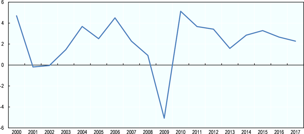
Source: OECD (2018[1]), Economic Outlook 103 - May 2018, https:/stats.oecd.org/index.aspx?DataSetCode=EO.
Productivity in Mexico, measured as GDP per hour worked, increased slowly over the 2000-16 period. Mexico’s productivity growth has recently picked up in sectors that benefitted from structural reforms: energy (electricity, oil and gas), financial and telecom (OECD, 2017[2]). Still, the gap with the OECD average has grown. The difference between labour productivity in Mexico and OECD countries rose from USD 24 in 2006 to almost USD 28 in 2016. Benchmarking productivity growth in Mexico with OECD member countries in the 2000-16 period puts the Mexican economy at the bottom of the ranking, just above Chile.
Resilient policy environmentw under changing external conditions
Despite 2017 being a challenging year for the Mexican economy, inflationary levels are stabilising now. Mexico has managed to reduce inflation since 2000 (Figure 1.2). However, uncertainty regarding the Trump’s administration policies – particularly the renegotiation of NAFTA – triggered an increase the interest rates that reached a historic high of MXN 22.04 per USD 1 in November 2016. In addition, the increase of gasoline prices caused a spike in inflation levels above the Central Bank’s target of 3% ±1.
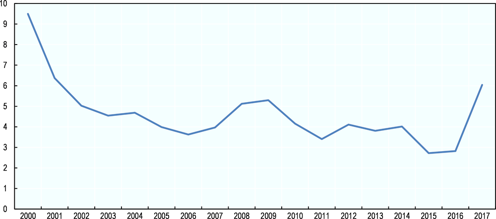
Note: Inflation is measured as changes in Consumer Price Index.
Source: OECD Statistics (2018[3]), Inflation (CPI), https://data.oecd.org/price/inflation-cpi.htm.
The large depreciation of the Mexican Peso (MXN) further increases the competitiveness of Mexican non-oil exports and has not pushed up inflation. Structural reforms are supporting a low inflation environment and strong expansion of credit, leading to gains in real wages and employment. It also has a positive impact on the fiscal balances, reflecting the USD-denominated oil receipts and the low exposure to foreign currency debt (OECD, 2017[2]). The so-called “Trump effect” also had its toll on investment. It decreased due to high interest rates and uncertainty regarding the outcomes of NAFTA negotiations. Foreign direct investment (FDI) in Mexico decreased by 5.8% in 2016. FDI increased by 11% in 2017 and appears to be on track towards recovery.
Growth has not been inclusive enough to achieve better living conditions for many Mexican families, as inequalities persist throughout the country. Regional disparities between a highly productive modern economy in the north and in the centre and a low-productivity traditional economy in the south have increased. In addition, income inequality in Mexico is the highest among OECD countries according to the latest data. The OECD Gini coefficient average in 2014 reached 0.318, while Mexico’s was 0.459.
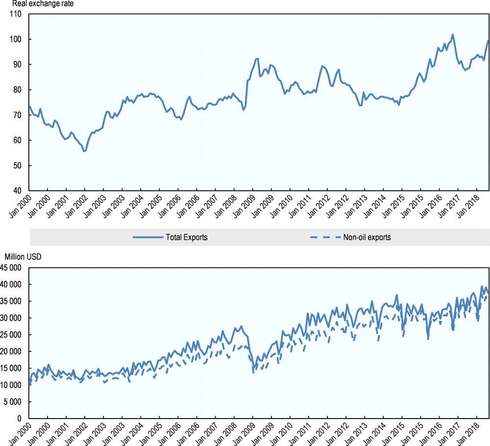
Sources: Banxico (2018[4]), Índice del Tipo Real de Tasa de Cambio, http://www.banxico.org.mx/SieInternet/consultarDirectorioInternetAction.do?sector=6&accion=consultarCuadro&idCuadro=CR60&locale=es; Banxico (2018[5]), Balanza Comercial, http://www.banxico.org.mx/SieInternet/consultarDirectorioInternetAction.do?accion=consultarCuadro&idCuadro=CE125§or=1&locale=es.
The state of territorial inequalities and population dynamics
Hidalgo, one of the 31 states and federal districts that compose Mexico, is located in the centre-east of the country. It borders Querétaro in the northwest, Veracruz in the northeast, San Luis Potosí in the north, Puebla in the southeast, Mexico in the southwest and Tlaxcala on the south. With a land area of 20 846 km² corresponding to 1.1% of the national land and a population of 2 858 359 inhabitants in 2015 corresponding to 2.4% of the national total, Hidalgo is one of the smallest states in Mexico (Figure 1.4). The state’s population density is 137 inhabitants per km², more than double the national mean (61 inhabitants per km²) and less than half that of Mexico City, the Federal District and Morelos.
The administrative divisions of state following OECD regional typology (see Box 1.1) include 13 TL3 regions, out of which: 2 are Predominantly Urban (PU); 4 are Intermediate (IN); 3 are Predominantly Rural Close to a City (PRCC); and 4 are Predominantly Rural Remote (PRR). In terms of national administrative boundaries, Hidalgo is divided into 84 municipalities with population sizes ranging from 2 667 to 277 375 inhabitants, 5 121 rural localities (with populations of less than 2 500 inhabitants) and 239 urban localities (with populations of 2 500 and over).
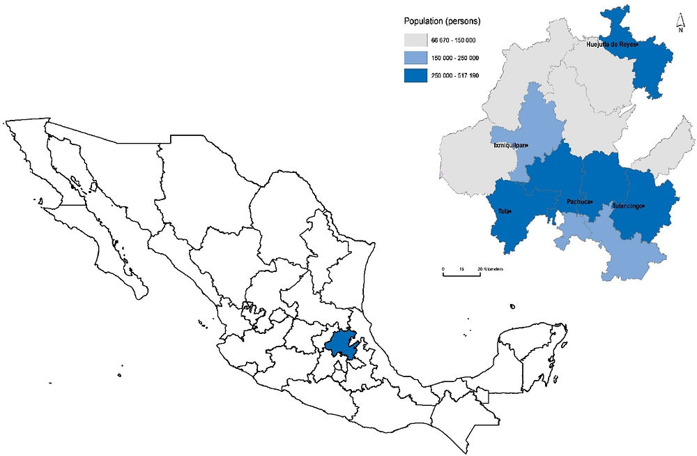
Note: Estimated population.
Sources: INEGI (2017[6]), Marco Geoestadístico Nacional; OECD (2018[7]), Regional Economy, OECD Regional Statistics (database), https://doi.org/10.1787/a8f15243-en.
Defining and classifying TL3 regions
The OECD regional database collects and publishes regional data at two different geographical levels, namely large regions (Territorial Level 2, TL2) and small regions (Territorial Level 3, TL3). Both levels encompass entire national territories. With some exceptions, TL2 regions represent the first administrative tier of subnational government (i.e. states in the United States, estados in Mexico, or régions in France). TL3 regions are smaller territorial units that make-up each TL2 region.
The OECD urban-rural typology classifies TL3 regions as “predominantly urban”, “intermediate” and “predominantly rural”. This typology is based on three criteria:
-
1. Identify rural local areas1 according to population density. A local area is defined as rural if its population density is below 150 inhabitants per km2 (500 inhabitants for Japan and Korea to account for the fact that the national population density exceeds 300 inhabitants per km2).
-
2. Classify regions according to the percentage of population living in rural local areas. A TL3 region is classified as predominantly rural if more than 50% of its population lives in rural local areas. TL2 regions are classified as predominantly urban if less than 15% of the population lives in rural local areas. If the share of the population in rural local areas is between 15% and 50%, it is categorised as intermediate.
-
3. Classify regions based on the size of the urban centres. Accordingly, a region classified as rural on the aforementioned basis becomes intermediate if it has an urban centre of more than 200 000 inhabitants (500 000 for Japan) representing no less than 25% of the regional population. A Tl3 region classified as intermediate on the aforementioned basis is classified as predominantly urban if it has an urban centre of more than 500 000 inhabitants (1 million for Japan) representing no less than 25% of the regional population.
The extended OECD typology developed in 2011 sub-divides rural TL3 regions further into 2 sub-categories: rural close to cities and rural remote by adding a distance criterion to urban centres according to a driving time threshold of 1 hour (45 minutes for North America) to the nearest population agglomeration of 50 000 inhabitants. Table 1.A.1 in Annex 1.A summarises the method.
In 2018, there were 389 TL2 and 2 251 TL3 regions across OECD countries.
← 1. A local area is the local administrative unit considered as the smallest building block for the classification. Being administrative entities, the average size of local administrative unit can change significantly across countries.
Source: Brezzi, Dijkstra and Ruiz (2011[8]), “OECD Extended Regional Typology: The Economic Performance of Remote Rural Regions”, https://doi.org/10.1787/5kg6z83tw7f4-en.
Hidalgo has a relatively large stock of working-age population...
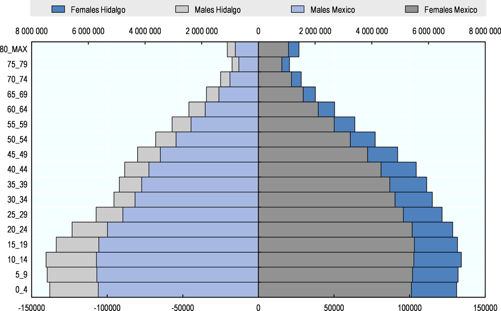
The population structure of Hidalgo currently ensures a relatively large stock of working-age population. The population pyramid of the state is wide at the bottom and gets smaller as age increases (Figure 1.5). As the percentage of the population outside working age is relatively small, the stock of human capital available in the economy is currently relatively large. The distribution of the population by gender and age groups in Hidalgo falls squarely into the national average.
In 2016, the percentage of the population in the broader youth, working-age and elderly categories (age ranges of 0 to 14, 15 to 64 (working age) and 65+ respectively) were 29%, 65% and 7% respectively, while for the OECD the respective shares were 18%, 66% and 18%. Compared to the national average, the only notable difference was a slightly lower share in the 15-64 year-old age group. The largest cohort of the population is in the 10-14 age range in Hidalgo as well as in Mexico, while it is in the 45-49 age range for the average of OECD countries. The proportion of females in total population was 51.7%, slightly higher than the national average of 51.2%.
Source: OECD (2018[7]), Regional Economy, OECD Regional Statistics (database), https://doi.org/10.1787/a8f15243-en.
National and international migrants feed the working-age population. Hidalgo is a net receiver of migrants from other Mexican states and has a long tradition of international migration to the United States. Between 2010 and 2015, inward migration to the state (of persons older than 5 years old) was 131 485, while outward migration was 77 176, for a net migration stock of 61 295 persons or 2.3% of the total population. Of the migrants that arrived in Hidalgo between 2010 and 2015, 77% were of working age, out of which 15% previously resided in the United States. To put this number in perspective, the United States hosted 97 out of 100 international migrants from Hidalgo in 2010 (INEGI, 2010[9]).
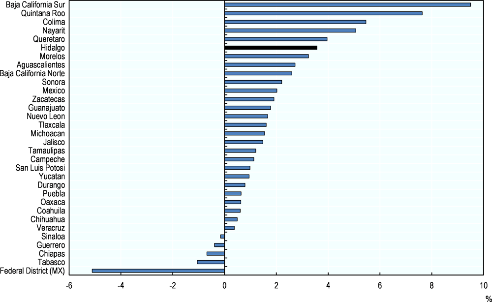
Amongst Mexican states, Hidalgo had the 6th largest net immigration flow as a percentage of total population in 2010 (Figure 1.6). As could be expected by geographical proximity and economic size, most of the inter-state migratory flows occur to and from places close to Hidalgo. In 2010, 71 out of 100 inward migrants came from the state of Mexico and Mexico City, while in 2005, 33 out of 100 outward migrants had these 2 places as a destination.
Source: OECD (2018[7]), Regional Economy, OECD Regional Statistics (database), https://doi.org/10.1787/a8f15243-en.
…that requires upskilling and more female participation
Despite recent improvements, the educational attainment levels of the working-age population remain lower than the national average. In 2015, 5% of the working population did not know how to read and/or write. Across educational levels, 22.3%, 54.9% and 22.3% had a primary, secondary and tertiary education as their highest completed educational level respectively. The average number of schooling years in 2015 was 8.7 years, slightly higher than in 2010 (8.1 years) and below the national average (9.2 years).
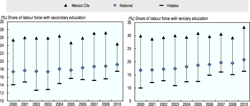
In Hidalgo, about 19% of children and adolescents of ages 3 to 15 do not have the mandatory level of education and do not attend any educational institution (CONEVAL, 2010[10]). Despite some improvement in 2010, there was no clear decreasing trend in the average secondary education gap of Hidalgo with respect to the national average between 2000 and 2010 (3.4 percentage points) and the top performing region, the Federal District (11 percentage points) (Figure 1.7). In terms of tertiary education, the average educational gap of Hidalgo’s working-age population between 2000 and 2010 was larger both with respect to the national average (5 percentage points) and to the Federal District (17 percentage points).
The gap in labour force participation between males and females in Hidalgo is wide for international standards. Female labour participation rates in Hidalgo are only half of their male counterpart: the rate was 77.7 for males and 38.6 for females in 2017. These low rates are in line with national trends, as women in Mexico are relatively much less likely to participate in the labour market than men in comparison to other OECD countries (OECD, 2017[11]).
Note: Data for 2009 not available.
Source: OECD (2018[7]), Regional Economy, OECD Regional Statistics (database), https://doi.org/10.1787/a8f15243-en.
The quality of the educational system in Hidalgo has improved in relation to other Mexican states but remains low for international standards. The 2017 results of PLANEA, a nation-wide test on language and mathematics, place Hidalgo above the national mean in basic secondary education and at the mean in higher secondary education. However, the OECD Programme for International Student Assessment (PISA) scores in mathematics, an international standard on the quality of the educational system, indicate there is room for improvement in the international context.
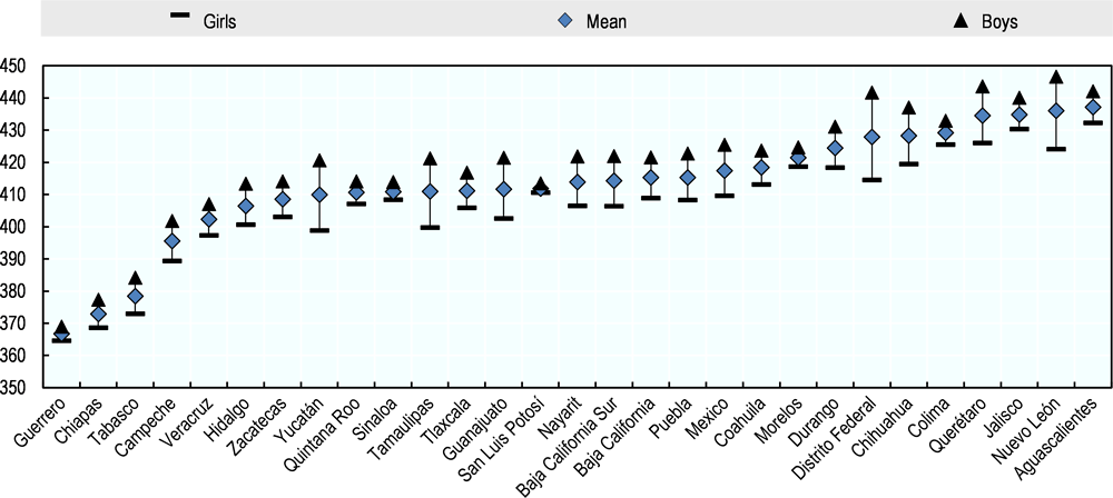
In terms of percentage of students with scores below Level 1 (the lowest value in the scale), Hidalgo occupies the 94th position amongst 133 regions worldwide scale, with 25% of students falling in this category. Among Mexican states, Hidalgo ranks at the 20th percentile in PISA scores in mathematics (Figure 1.8). In line with national average values, the standard variation in scores in Hidalgo is 74, which indicates a relatively large variation in performance across schools in the state.
The gender educational gap in Hidalgo, as measured by standardising international scores, is wide. The gap between boys and girls scores in Hidalgo is statistically significant, although not as large as in other states such as Jalisco and Yucatán (Figure 1.8).
The next decades will bring about population ageing and stabilisation in the increase in activity rates. Although the gap between the youth dependency ratio of Hidalgo and the OECD average was still considerable in 2016 (16 percentage points), there is a clear decreasing trend over time, in line with national trends (Figure 1.9). This decrease implies a steady increase in the median age over time, which stood at 27 years in 2015. The demographic transition experienced by Hidalgo over the last decade from the young cohort to the working-age cohort resulted in a rapid increase in the activity rate towards the OECD average. The steady increase in the activity rate, together with the medium-term increase prospects given the current size of the 10-14-year cohort, translates into opportunities for utilising human capital in production, but also into growing pressures on job creation in the labour market.
Note: The difference between boys and girls scores for Hidalgo is statistically significant.
Source: OECD (2014[12]), PISA 2012 Results: What Students Know and Can Do (Volume I, Revised edition, February 2014): Student Performance in Mathematics, Reading and Science, https://doi.org/10.1787/9789264208780-en.
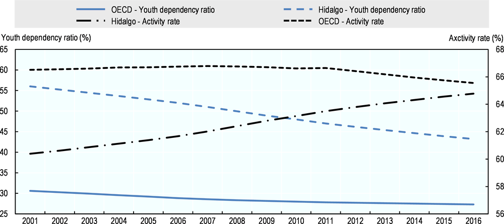
Note: Youth dependency ratio is calculated as the population less than 15 years over the total population; activity rate is the ratio of the working-age population (+15 – 64) over total population.
Source: OECD (2018[7]), Regional Economy, OECD Regional Statistics (database), https://doi.org/10.1787/a8f15243-en.
The rural-to-urban transition is not yet complete
The majority of Hidalgo’s population resides in rural localities outside metropolitan areas. Six of the 13 TL3 regions of Hidalgo have populations smaller than 160 000 inhabitants. These sparsely populated areas are located in mountainous regions with difficult access, as indicated by their high ruggedness of terrain index values (Figure 1.12). The percentage of the population in urban areas of 15 000 inhabitants or more was 28.8% in 2015. The reminding population was split in 23.6% in mixed localities (with populations above 2 500 and below 15 000) and 47.6% in rural localities. According to the OECD regional typology, which is based on population density thresholds at the local area level, in 2010 Hidalgo recorded a lower percentage of population in urban and rural areas than the national average (14% versus 46%, and 26% versus 37% respectively) and a higher percentage of the population in intermediate areas (60% versus 17%) (Figure 1.10).
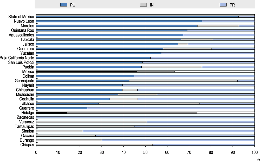
Note: “PU” refers to predominantly urban area, “IN” refers to intermediate areas and “PR” predominantly rural area.
Source: OECD (2018[7]), Regional Economy, OECD Regional Statistics (database), https://doi.org/10.1787/a8f15243-en.
A long-term comparison of urbanisation rates with other Mexican states reveals that current urbanisation rates are much lower than what would be expected by Hidalgo’s size and level of development. Unlike other roughly comparable states at the beginning of the period in 1950 such as Querétaro and Puebla, urbanisation rates in Hidalgo did not take off in the 1960s and 1970s (Figure 1.11). The underlying reasons for slower urbanisation rates include stronger incentives to remain in rural areas and agricultural activities than outweighed the benefits of migrating to cities. Among these, low expected urban wages and targeted subsidies that narrowed rural-to-urban work income differentials may have played a defining role in maintaining a significant percentage of the population in low-density areas.
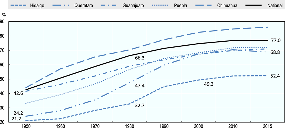
Note: Urbanisation rate defined as percentage of urban population in total.
Sources: INEGI (2010[13]), Censo de población 2010; INEGI (2017[14]), Encuesta Intercensal 2015.
The metropolitan areas of the capital city of Pachuca de Soto (hereafter Pachuca), Tula and Tulancingo are located in southern plains concentrating most of the economic development of the state. The 3 areas form an arch, above which the largest urban agglomeration is Huejluta de Reyes with a population of about 130 000. The north has mostly high altitudes and relatively dispersed population (Figure 1.4 and Figure 1.12).
The fast-growing metropolitan area of Pachuca is relatively small for Mexican standards. The metropolitan area of the state capital Pachuca, with a population of 646 880 inhabitants in 2014, is the most populated urban centre. Pachuca ranks in the bottom 3 in terms of size amongst 33 metropolitan areas in Mexico. In terms of population growth, it recorded a relatively high annual average population growth rate of 3.5% in the 2000-14 period, above the national average of 2.5% and the second largest amongst metropolitan areas below 1 million inhabitants (Figure 1.13). The state capital is located at less than 100 km from the heart of the Valley of Mexico Metropolitan Area, the largest conurbation of Mexico with a population of over 20.4 million inhabitants.
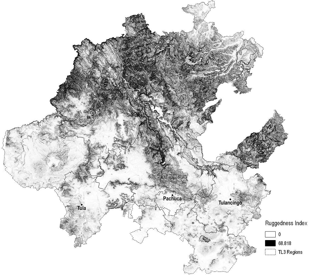
Notes: 30m underlying digital elevation model resolution.
Darker shades indicate higher terrain ruggedness.
Source: INEGI (2013[15]), Continuo de Elevaciones Mexicano (CEM 3.0) (Accessed July 2018) http://www.beta.inegi.org.mx/app/geo2/elevacionesmex/
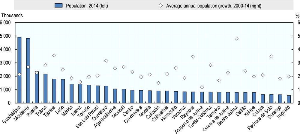
Note: For visual purposes, the figure excludes the largest metropolitan area (Mexico City).
Source: OECD (2018[7]), Regional Economy, OECD Regional Statistics (database), https://doi.org/10.1787/a8f15243-en.
Under current inequalities in accessibility, opportunities will likely remain concentrated around urban areas
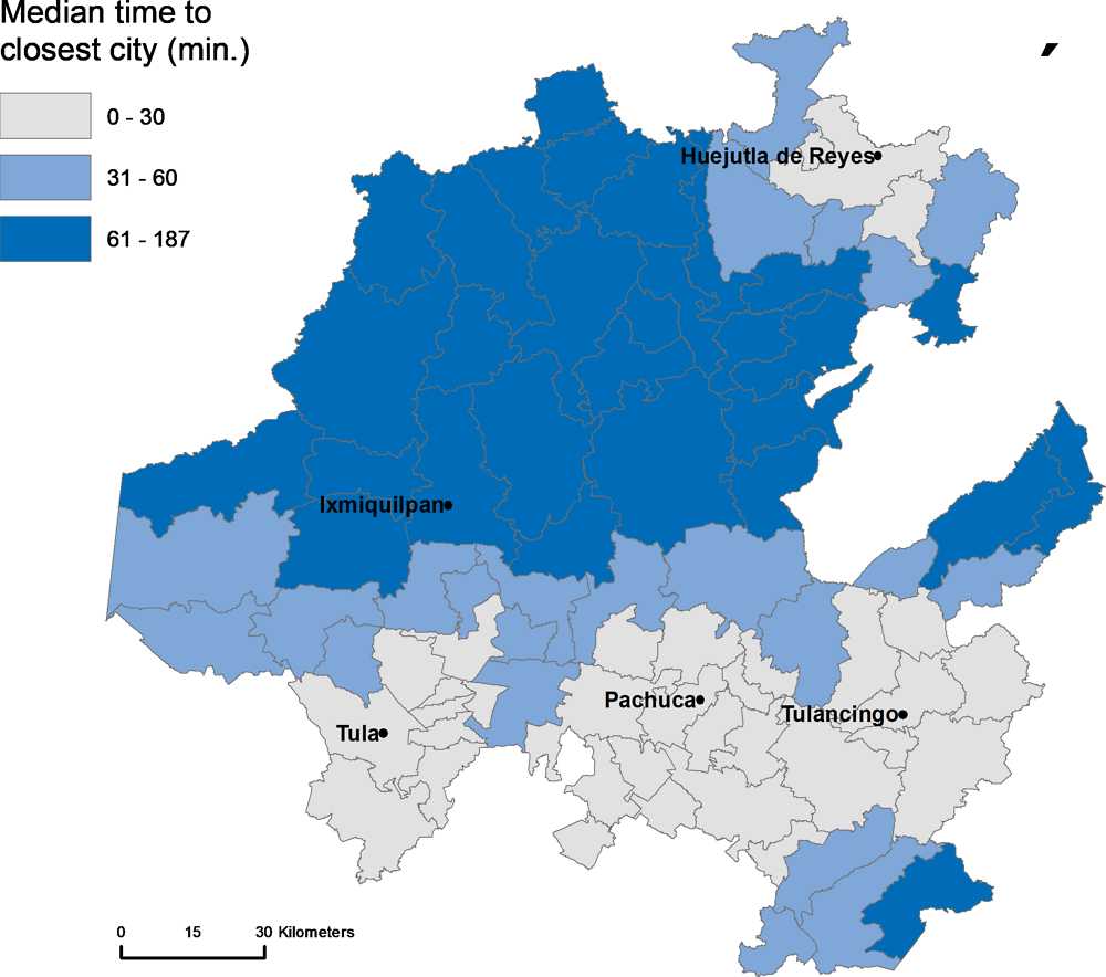
Accessibility, or the ease with which people in different locations can physically access markets – for goods, services and employment and business opportunities – is highly unequal within the state. Figure 1.14 shows the median time needed by municipality to reach a city of at least 50 000 people using the fastest mean of transport available in each 1-km² grid cell (for methodological details see Annex 1.B). Municipalities surrounding the main cities (Tula, Pachuca, Tulancingo) and the smaller urban settlement of Huejluta de Reyes in the north can access at least 1 city both within and outside the state in neighbouring states of Tlaxcala and San Luis Potosí within a 30-60-minute journey. In contrast, municipalities with the worse performance in terms of access are found in between these rings: in municipalities in the northwest such as La Misión, Pacula and Tlahuiltepa, it takes more than a 2-hour journey to reach any city of at least 50 000 inhabitants.
Notes: See Annex 1.B for details on the measurement of accessibility.
Median time calculated from 1-km2 grid cells
Sources: Weiss et al. (2018[16]), “A global map of travel time to cities to assess inequalities in accessibility in 2015”, https://doi.org/10.1038/nature25181; INEGI (n.d.[17]), Conjunto de Datos Vectoriales de Carreteras y Vialidades Urbanas Edición 1.0 (Distribución por Entidad Federativa), http://www.inegi.org.mx/geo/contenidos/topografia/vectoriales_carreteras.aspx.
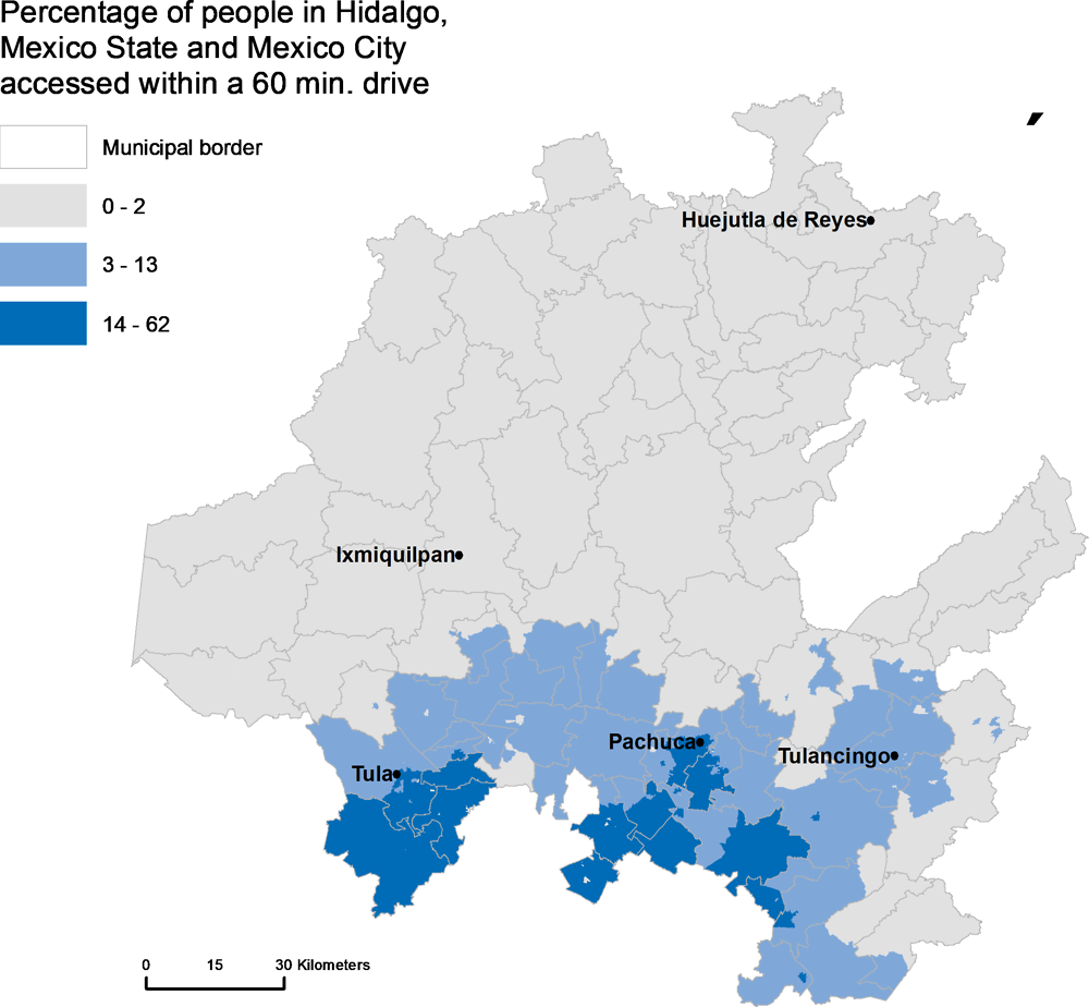
Access to the combined markets of Hidalgo, Mexico State and Mexico City is also highly unequal across the state. Figure 1.15 shows the share of the population reachable within a one-hour drive from any locality in the state. While the most accessible localities bordering Mexico State in the south can access 62% of the combined population of Hidalgo, Mexico State and Mexico City within a 1-hour drive, all localities in the north and some localities in the east and west can access less than 2%. In absolute terms, this means that after driving for 1 hour a person in a locality with low accessibility can reach as little as 526 people, while a person in the most accessible locality can access over 17 million people.
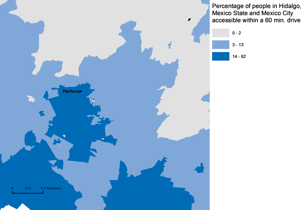
Geographic, human settlement patterns and physical infrastructure are behind unevenness in accessibility. Because areas with more difficult terrain pose higher road provision costs, geography largely determines accessibility, as indicated by the match between areas with low ruggedness in Figure 1.12 and areas with high accessibility in Figure 1.15. Geographical conditions also determine the initial location of human settlements. Once established, urban centres tend to grow, giving urban areas a self-sustained advantage in terms of accessibility. This is evident in the presence of large disparities in accessibility even within urban areas (Figure 1.16). The last part of the story is physical infrastructure. Its provision usually serves the most pressing connectivity demands in terms of absolute number of flows, leaving remote and less transited places disconnected from the main transport networks.
Note: See 0 for details on the measurement of accessibility.
Sources: Open Street Maps (2018[18]), database (accessed July 2018) https://www.openstreetmap.org; INEGI (n.d.[17]), Conjunto de Datos Vectoriales de Carreteras y Vialidades Urbanas Edición 1.0 (Distribución por Entidad Federativa), http://www.inegi.org.mx/geo/contenidos/topografia/vectoriales_carreteras.aspx; INEGI (2010[13]), Censo Poblacional 2010.
Sources: Open Street Maps (2018[18]), database (accessed July 2018) https://www.openstreetmap.org; INEGI (n.d.[17]), Conjunto de Datos Vectoriales de Carreteras y Vialidades Urbanas Edición 1.0 (Distribución por Entidad Federativa), http://www.inegi.org.mx/geo/contenidos/topografia/vectoriales_carreteras.aspx;
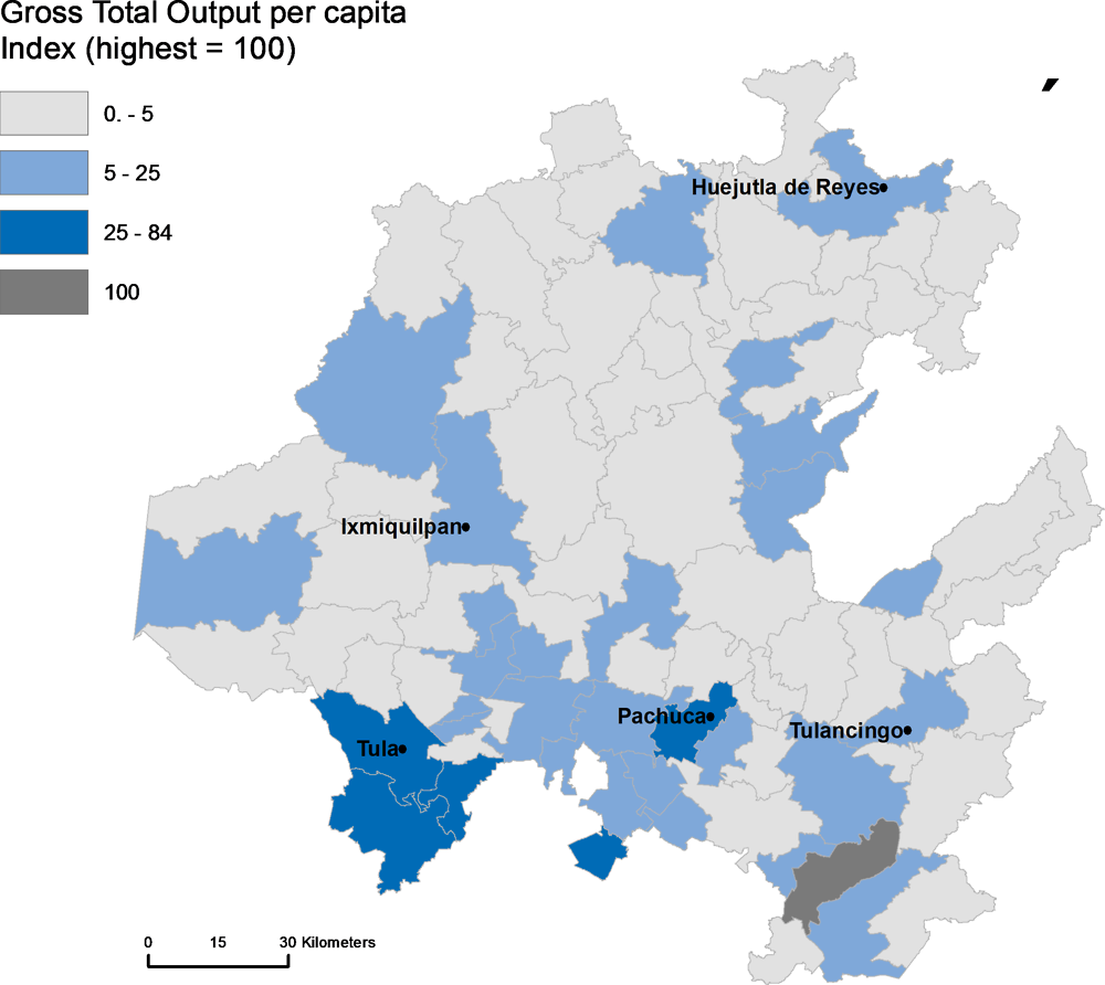
The territorial distribution of economic activity in Hidalgo is highly concentrated and shows a strong north-south divide. The distribution of gross total output per head in 2014 across municipalities is highly unequal (Figure 1.17). In most municipalities, gross total output per head was only one-fifth of the municipality with the highest value, Tepeapulco, which has a strong manufacturing base. In the north, most municipalities’ total output per head is less than 5% of Tepeapulco’s, indicating a rather thin economic base outside a handful of municipalities in the south around Tula and Pachuca.
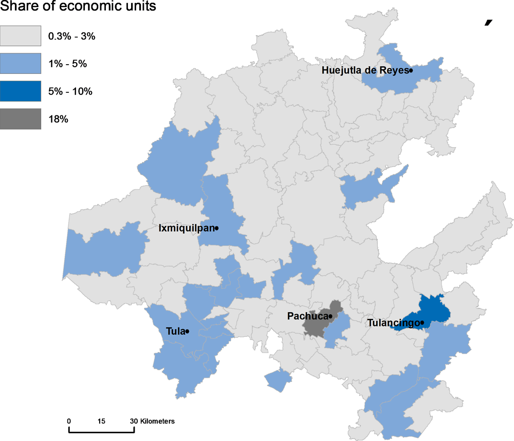
Disparities in accessibility reinforce a highly uneven distribution of businesses across municipalities. The index of geographic concentration1 across municipalities is 39.5 when calculated for population and 50 when calculated over businesses, indicating that economic activity is far more concentrated than population. Half of all businesses are concentrated in just 7 municipalities, with Pachuca alone concentrating 18% of all the economic units of the state (Figure 1.18). The strong north-south divide in population is even more marked in terms of economic activity. The major urban areas outside the southern area, Ixmiquilpan and Huejutla de Reyes, concentrate only 4.5% and 4.6% of all businesses in Hidalgo respectively.
Sources: INEGI (2015[19]), Economic census 2014; INEGI (2017[14]), Encuesta Inter-censal 2015.
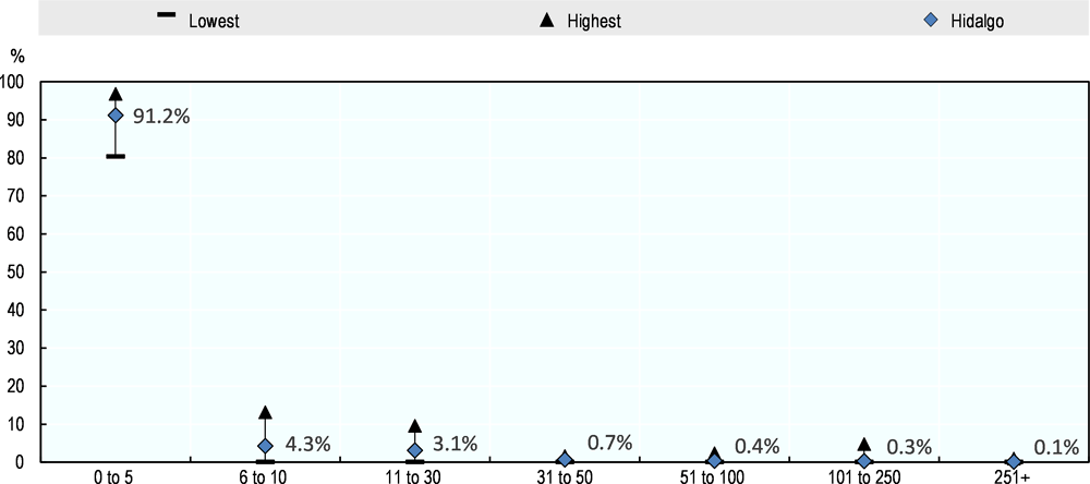
While most businesses in Hidalgo are microenterprises, the small and medium business sector has little weight and is geographically concentrated. The distribution of businesses by size class across municipalities is highly skewed towards small size establishments (Figure 1.19). In 2013, the overwhelming majority of businesses across municipalities in Hidalgo were micro-enterprises with less than ten employed persons. In fact, more than half of total employment is in micro-enterprises, while the share of employment in small and medium businesses (employing between 11 and 250 persons) was 28% (INEGI, 2015[19]).
The share of employment in businesses with 5 employed persons or less varied from 80% to 98% across municipalities, with an average value of 91%. The share of businesses by size class and its geographical variation decrease abruptly for larger sizes. In fact, 28 out of 84 municipalities registered 0 businesses with 31 to 50 employed persons. This number increases to 50 out of 84 in the 51 to 100 employed category, indicating that the small and medium business sector is not only small but also geographically concentrated.
Source: INEGI (2017[20]), Directorio Estadístico Nacional de Unidades Económicas (database).
Source: INEGI (2015[19]), Economic census 2014.
Unlocking economic development through structural change
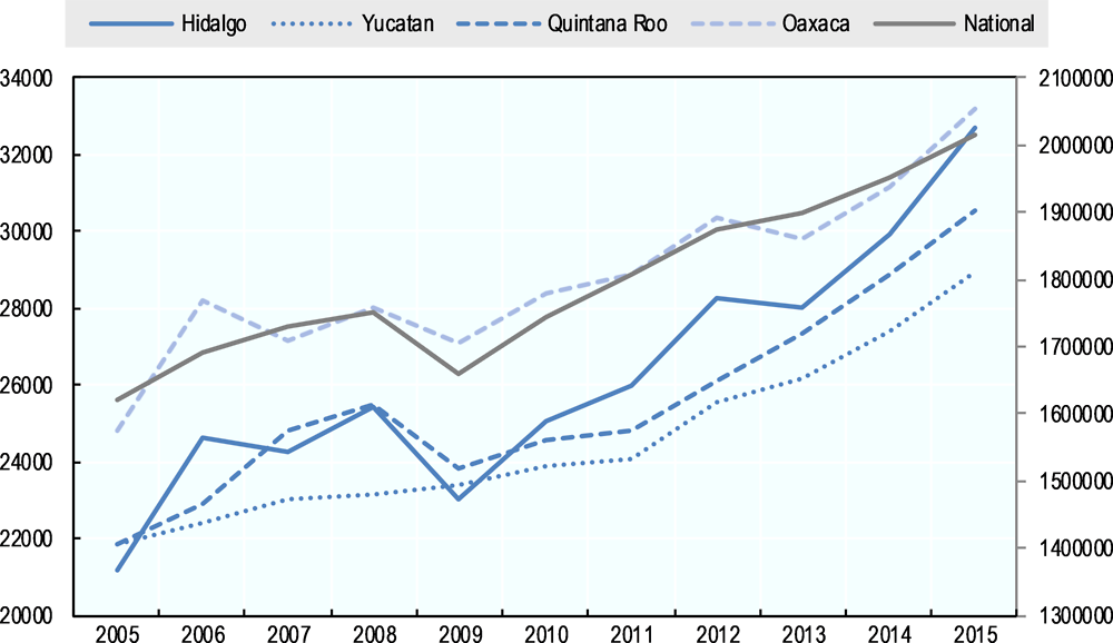
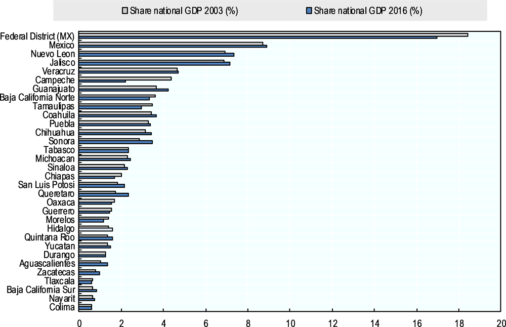
Hidalgo’s economic size and its share in the national economy increased in the past decade. Hidalgo’s GDP stood at USD 32 613 billion in 2016, about a third more than in 2005 (Figure 1.20). The expansion in economic size took off in the aftermath of the financial crises in 2008-09 at a stronger pace than states of initial comparable size such as Yucatán, and Oaxaca, with a notable acceleration in the period 2013-16. The strong performance in terms of GDP has translated into a larger contribution of Hidalgo to the national GDP, from 1.38% in 2003 to 1.57% in 2016, ranking as the 21st largest among the 32 TL2 units in Mexico, 2 positions above 2003 levels (Figure 1.21).
Hidalgo’s full growth potential has yet to be realised
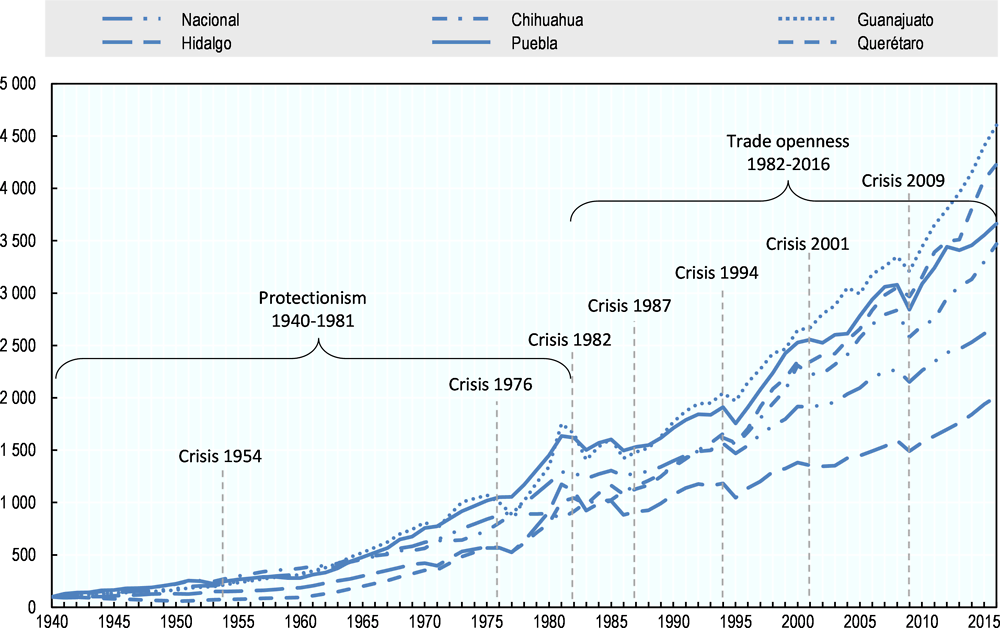
Hidalgo’s GDP per capita stood at USD 11 195 in 2016, the 25th largest amongst Mexican TL2 regions. Historically, the gap in GDP between Hidalgo and comparable Mexican TL2 regions became wider in the period of trade liberalisation that started in the early 1980s (Figure 1.22). Growth after the last of a series of economic crises in 2008 accelerated, although at a slower pace than in other states such as Guanajuato, Querétaro and Chihuahua.
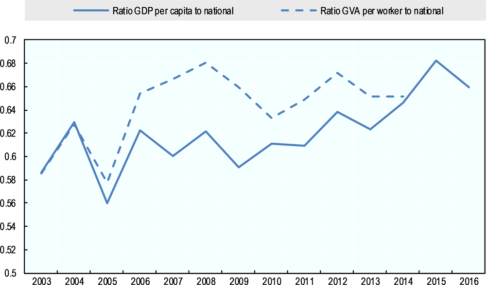
Hidalgo has been catching up with the national average over time albeit at a moderate pace. The ratio of Hidalgo’s GDP per capita to the national average was 0.66 in 2016, up from 0.59 in 2003, thanks to faster catching-up trends in the 2010-15 period (Figure 1.23). Average labour productivity, measured as gross value added (GVA) per worker, stood at USD 27 390, the 20th largest amongst Mexican TL2 regions. In terms of labour productivity growth, Hidalgo registered an average growth rate of 3% in the 2010-15 period, the 6th largest across Mexican TL2 regions. The gap in terms of worker productivity, measured by the ratio of GVA per worker over the national average stood at 0.65 in 2014, slightly higher than in 2010.
Hidalgo’s productivity levels across all industries rank around the bottom 5% across OECD regions, and in the top 25% in manufacturing (Table 1.1). GDP per worker in Hidalgo in 2014 was the 29th lowest amongst 385 OECD regions, above regions in Bulgaria, Chile, Colombia, Mexico and Romania. The absolute gap in terms of GVA per worker with respect to the median of OECD regions was USD 37 939. Hidalgo occupies a higher place in terms of productivity per worker in the manufacturing sector, ranking 238th among 290 OECD regions, with levels above regions in Bulgaria, Chile, Greece and Portugal, among others.
Note: In constant USD 2010. Secondary axis used to represent national values.
Source: OECD (2018[7]), Regional Economy, OECD Regional Statistics (database), https://doi.org/10.1787/a8f15243-en.
Source: OECD (2018[7]), Regional Economy, OECD Regional Statistics (database), https://doi.org/10.1787/a8f15243-en.
Source: INEGI (2015[19]), Economic census 2014; German-Soto Vicente (2017[21]), Generación del Producto Interno Bruto Mexicano por Entidad Federativa, 1940-1992.
Note: GVA per worker calculated using employment by place of residency (GVA and employment values for 2015 not available).
A value of 1 indicates no gap with the national average.
Source: OECD (2018[7]), Regional Economy, OECD Regional Statistics (database), https://doi.org/10.1787/a8f15243-en.
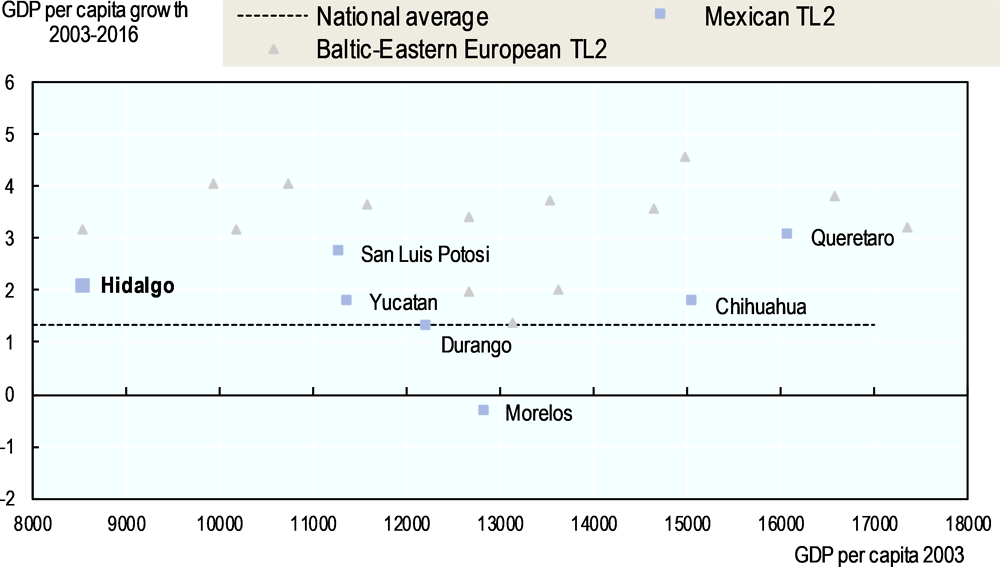
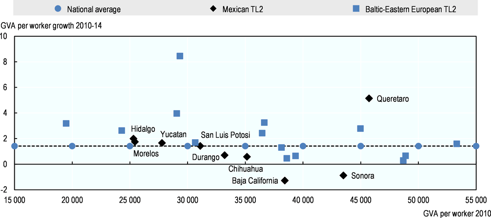
Although Hidalgo’s economy performed strongly in the national context, a comparison with similar OECD regions reveals there is room to access untapped resources. Hidalgo’s performance in terms of GDP per capita growth over the 2003-15 period was relatively high compared to other Mexican states, but relatively low with respect to comparable OECD regions.
Hidalgo registered a GDP per capita growth rate of 2.11% in the 2003-16 period, above similar states such as Durango, Morelos and Yucatán and the national average of 1.01% (Figure 1.24). In the meantime, the top performing state of Querétaro, San Luis Potosí and 11 out of 15 comparable non-Mexican regions grew at a faster rate, with top performing regions registering growth rates as high as 4.6% in the same period.
The situation is similar with respect to GVA per worker in the 2010-14 period, during which Hidalgo registered a growth rate of 2%, in line with most of the comparison group of OECD regions (Figure 1.25). Hidalgo’s labour productivity growth rate was the second largest amongst comparable Mexican states, behind the impressive 5% growth rate of Querétaro.
Source: OECD (2018[7]), Regional Economy, OECD Regional Statistics (database), https://doi.org/10.1787/a8f15243-en.
Source: OECD (2018[7]), Regional Economy, OECD Regional Statistics (database), https://doi.org/10.1787/a8f15243-en.
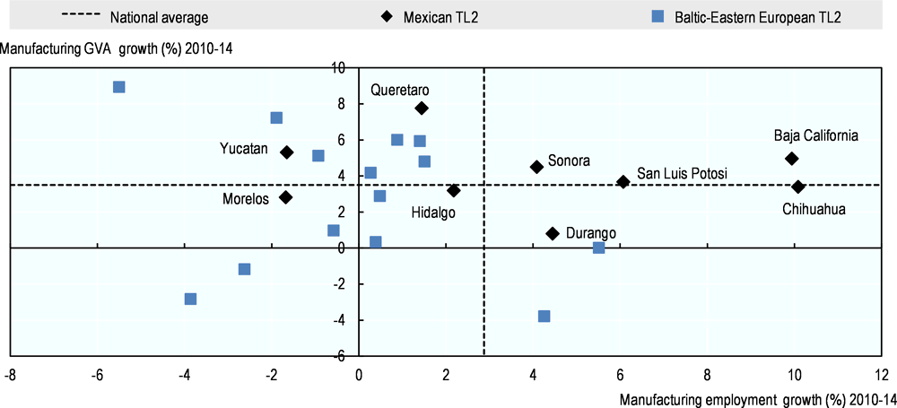
The manufacturing sector could be an engine of growth in Hidalgo if employment growth keeps pace with the sector’s expansion. The comparison of manufacturing GVA growth against employment growth is indicative of the labour generation capacity of the manufacturing sector. High GVA growth rates accompanied by slow employment growth rates over a given period are a symptom of a highly capital-intensive manufacturing sector with little labour absorption capacity. While Hidalgo registered manufacturing GVA and employment growth rates below the national average, most comparable Mexican states registered high rates of both GVA and employment in manufacturing (Figure 1.26). An extreme version of the situation where manufacturing GVA expands while manufacturing employment declines is visible in other comparable Mexican states such as Yucatán and Morelos, and several other comparable OECD regions.
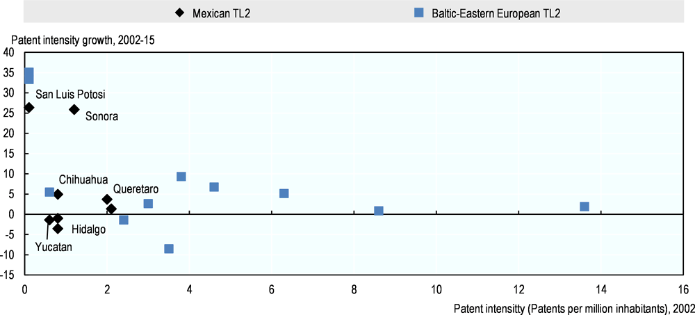
Transitioning towards sectors with higher technological content will be difficult unless there is an explicit strategy to address current innovation gaps. The innovation performance of Hidalgo in the national and international context is relatively poor and has not improved over time. The number of patents per million inhabitants in Hidalgo was 0.5 in 2015 and 0.8 in 2002, indicating that innovation performance as fared by this measure has worsened over time. Meanwhile, the average of Mexican states increased from 1.2 in 2002 to 2.8 patents per million inhabitants in 2015. Hidalgo lagged behind comparable Mexican states such as San Luis Potosí and Chihuahua that started from a comparatively small patenting base in 2002. Other OECD regions with a similar economic structure in Baltic and East European countries had a stronger basis for technological transition even in 2002.
Source: OECD (2018[7]), Regional Economy, OECD Regional Statistics (database), https://doi.org/10.1787/a8f15243-en.
Source: OECD (2018[7]), Regional Economy, OECD Regional Statistics (database), https://doi.org/10.1787/a8f15243-en.
Tertiarisation will continue shaping a diversified economic structure
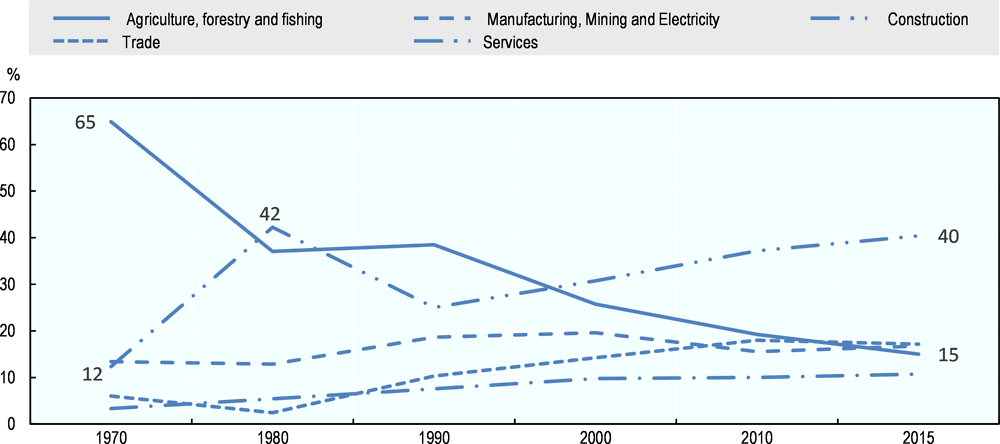
Hidalgo has a diversified economic structure, with a relatively high but declining share of manufacturing. The share of occupied population over total in manufacturing, mining and electricity sectors has remained relatively stable since 1970, while the service sector exploded at the expense of the agricultural sector since the 1990s (Figure 1.28). The share of occupied population in manufacturing, mining and electricity declined by 3 percentage points since 2000 to reach 17% in 2015.
Sources: INEGI (2010[13]), Censo de población 2010; INEGI (2017[14]), Encuesta Intercensal 2015.
By 2015, manufacturing and distributive trade, repairs and other activities explained over half of the state’s GVA (Table 1.2). The share of tradable goods and services in total GVA was 36% in 2015, 2 percentage points below the national average and down from 53% in 2004.
Hidalgo does not have a particularly specialised productive structure and has become more diversified over time. The state’s Specialisation Index measures how similar the state productive structure is with respect to the national average. The index indicates whether sectors are over- (larger than 1) or under-represented (smaller than 1) with respect to the national average. According to this measure, Hidalgo has one of the lowest levels across Mexican states (Figure 1.29). In line with national trends, specialisation levels in Hidalgo decreased between 2004 and 2015. With respect to the national composition, in 2015 construction (1.30) and manufacturing (1.27) were the most over-represented sectors, while information and communication (0.20), professional, scientific, technical activities, administrative, support service activities (0.27), financial and insurance activities (0.52) and were the most under-represented.
Notes: The index is calculated as the sum of the absolute values of the difference between the share of each sector and the corresponding national average, with 0 indicating that the economic structure of the state is the same as the national and 2 indicating an entirely different structure (the maximum value is calculated as 2(I-1)/I, where I = 11 industries).
Higher values of the index indicate higher sectoral specialisation.
Source: OECD (2018[7]), Regional Economy, OECD Regional Statistics (database), https://doi.org/10.1787/a8f15243-en.
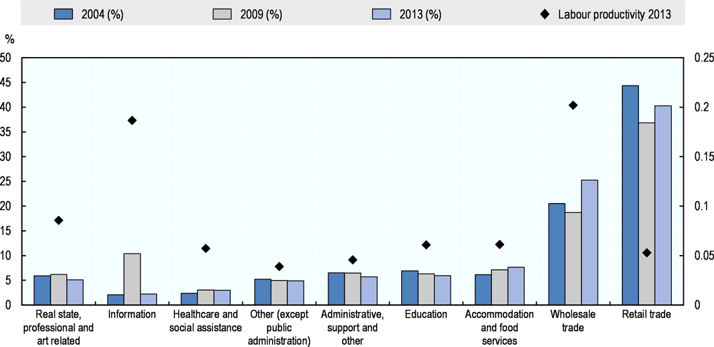
Low productivity non-tradable service activities have considerable weight in the service sector of Hidalgo. The service sector GVA is dominated by retail and wholesale activities, that together in 2014 had a combined share of 65% of GVA in the service sector (Figure 1.30). Over 60% of GVA in services is produced in non-tradable sectors, which include healthcare and social assistance, administrative and support activities, education, accommodation and food services, wholesale trade and retail trade and other services.
The evolution in the composition of the service sector over time does not indicate a clear trend towards tradable service activities. Tradable services have gained momentum as complements to manufacturing in international markets. In Hidalgo, there are no visible signs of increasing specialisation in tradable services besides an increase in the share of the wholesale trade sector in the 2004-13 period (Figure 1.30). Labour productivity, measured as output per hour, is on average 2.6 times lower in the non-tradable sector compared to the average of the tradable sector. Labour productivity in retail trade, the sector with the highest participation in terms of GVA, is the third lowest amongst service activities.
Note: Labour productivity is calculated as total production (in current MXN) over hours worked.
Source: INEGI (2015[19]), Economic census 2014.
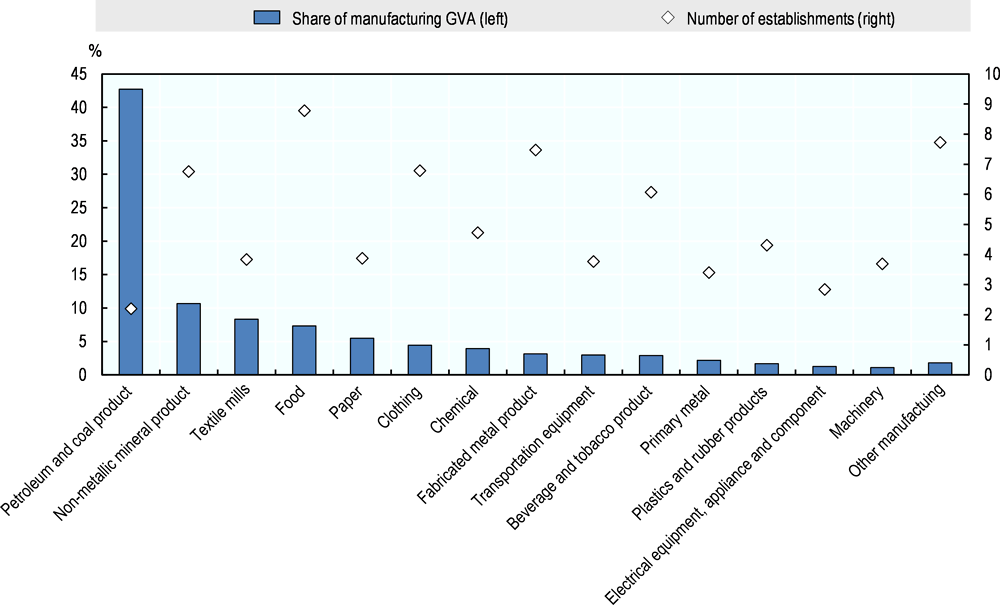
A considerable share of manufacturing value added has relied on an industry with strongly limited potential for spill-overs to small and medium enterprises and other industries. The petroleum and coal products industry share in total GVA was 43% in 2013, sharply increasing its participation from 17% in 2008 (Figure 1.31). The next industries in importance were the non-metallic mineral products (10%), textile mills (8.3%) and food (7.3%) sectors, which respectively had 805, 36 and 5 616 establishments in 2014. In the petroleum and coal products industry, there were only 8 registered establishments in 2013, a much lower value compared to the state average of 564 establishments across industries.
With its exceptionally high concentration in terms of establishments, the most important sector in terms of GVA currently integrates only a few small and medium-sized enterprises. Furthermore, according to the national input-output matrix for 2013, 73% of the inputs of the petroleum and coal products industry come from the gas and petroleum industry, which evidences the industry’s low upstream spill-over potential in the value chain.
Note: The establishment count by sector displayed in natural logarithms.
Source: INEGI (2015[19]), Economic census 2014.
Investment volatility hinders the consolidation of key manufacturing sectors
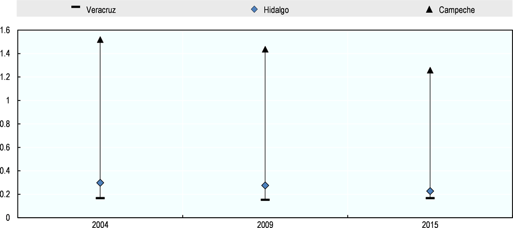
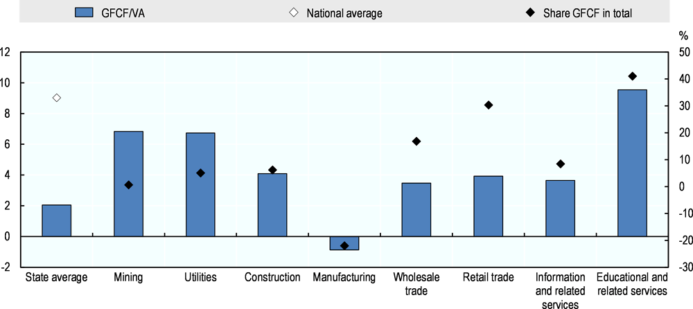
Specialisation in oil-related industries partly explains a loss in the capacity to attract investment to the state within the national context between 2004 and 2013. Total investment, defined as the change in assets, inputs and products within a period, was 3.6% of the total value added in 2013, around one-third of the national average (Figure 1.32). Total investment in fixed assets, or gross fixed capital formation, as a share of total value added, was 2.06% in 2013, down from 11% in 2004 and 15% in 2009.
The gap with the national value, which in 2013 was of around 7 percentage points, indicates that Hidalgo had relatively low capacity to attract investment in fixed assets. This was due partly because of a substantial drop in oil-related manufacturing investment. The breakdown of total investment in fixed assets as a percentage of value added indicates that the manufacturing sector – and more specifically the manufacturing of products derived from oil and charcoal – took a severe hit over the period, which even turned negative its share in total investment in fixed assets across sectors. This share was 51% in 2009, which gives an indication of the large volatility of investment in fixed assets.
Foreign direct investment (FDI) flows have fluctuated widely over time. Total FDI flows to Hidalgo amounted to USD 357 million in 2017 and accumulated to about USD 4 000 million between 1999 and 2017 (Figure 1.33). In 2015, 1.5% of the total FDI to Mexico went to Hidalgo, placing the state 17th amongst 32 states and federative units. Over the 1999-2017 period, FDI flows have not shown a steady increase over a sustained period and have instead fluctuated around a mean value of USD 52 million. This pro-cyclical behaviour is also present in states one position above (Morelos) and one position below Hidalgo (Oaxaca) in terms of participation in total national FDI flows by state.
GFCF: Gross fixed capital formation.
VA: Total value added
Notes: Agriculture’s share in total gross fixed capital formation in 2014 was 0.7%. Information-related services include finance and insurance, real estate and rental and leasing, professional, scientific and technical services, management of companies and enterprises, administrative and support and waste management and remediation services.
Gross fixed capital formation is the change in investment in fixed assets (machinery, property, etc.).
Source: INEGI (2015[19]), Economic census 2014.
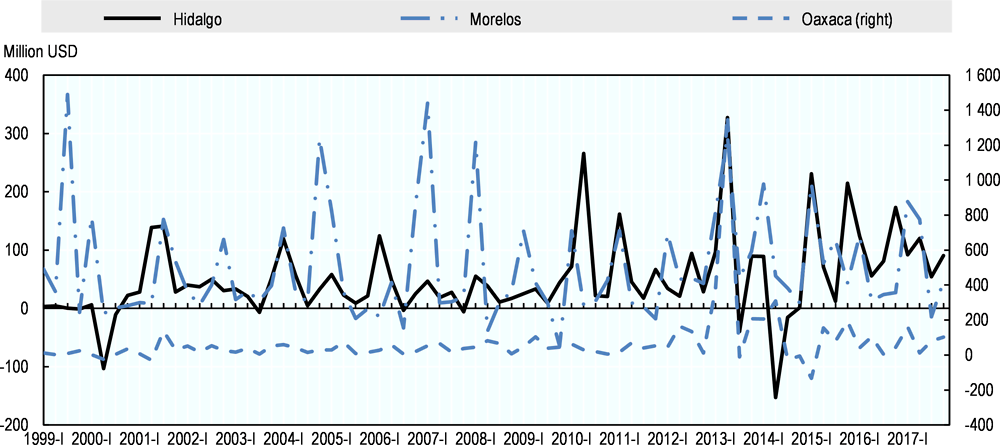
Source: National Registry of Foreign Investment (2018[22]), Secretary of Economy, (accessed August 2018) https://www.gob.mx/se/acciones-y-programas/competiti.
Foreign Direct Investment (FDI) has mostly originated in the United States and has concentrated in manufacturing. Across countries, 40% of FDI flows to Hidalgo between 1999 and 2017 came from the United States, 19% from Canada, 15% from Spain and the remaining 25% from other countries. However, in recent years, FDI from United States has reduce its relevance within Hidalgo, falling to a share of 23% of total FDI between 2008 and 2017, below the average at national level (43%). Across sectors in the 1999-2017 period, the largest share went to the manufacturing sector (44%), followed by transport (18%) and financial services and insurance (14%). The main subsector in terms of FDI in Hidalgo in the 1999-2017 period was beverages and tobacco, which accounted for 41% of manufacturing FDI. Other states disproportionally attracting FDI in this subsector include comparable states such as Chiapas, Oaxaca and Yucatán.
Ensuring stable, secure and well-paid jobs
Hidalgo’s labour market is split between formal and informal segments. The informal sector comprises employment outside legal regulations in formal and informal productive establishments producing legal goods and services (Jütting and de Laiglesia, 2009[23]). The formal sector of Hidalgo absorbed only 24% of total employment in 2017, despite an increase in formal employment of 45% over the 2004-14 period.
Formal employment opportunities are concentrated in service sectors in urban areas
The distribution of the change in formal employment between 2004 and 2013 across municipalities was highly uneven. Out of 110 000 net new formal jobs in the period, almost 30% were concentrated in the adjacent municipalities of Pachuca and Mineral de la Reforma (Figure 1.34). The correlation between employment levels in 2004 and the share in the change in employment growth in 2004-13 was 85%, clearly indicating the consolidation of larger employment centres over the period and the relative loss of importance of thinner labour markets. The spatial distribution of employment creation clearly indicates the attractiveness of the southern corridor in the form of an arch starting from Apan in the southeast, traversing Pachuca in the south centre and ending in Tula de Allende in the southwest.
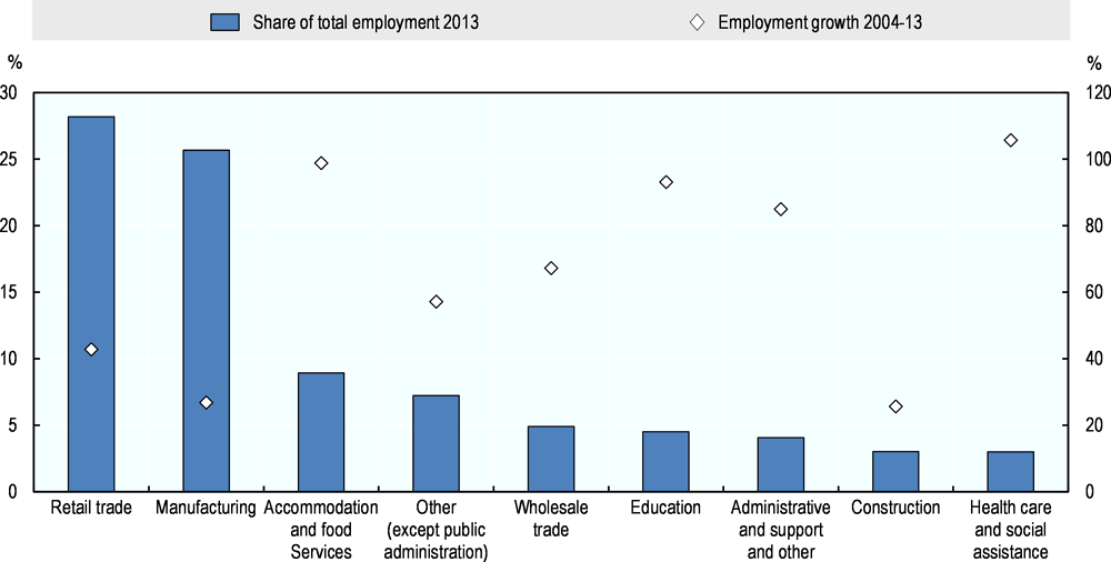
Most formal employment in Hidalgo remains concentrated in retail trade and manufacturing, despite a significant expansion of non-tradable service activities. Retail trade and manufacturing absorbed each about one-quarter of total formal employment in Hidalgo in 2014 (Figure 1.35). Most activities registered an increase in employment over the period, except for agriculture, electricity and finance, and insurance, further reducing their already small share in total employment. Formal employment creation in service activities was on average more dynamic than the manufacturing sector. Accommodation and food services had the most notable performance across sectors, doubling its level of employment in the 2004-13 period to become the 3rd most important sector in 2013.
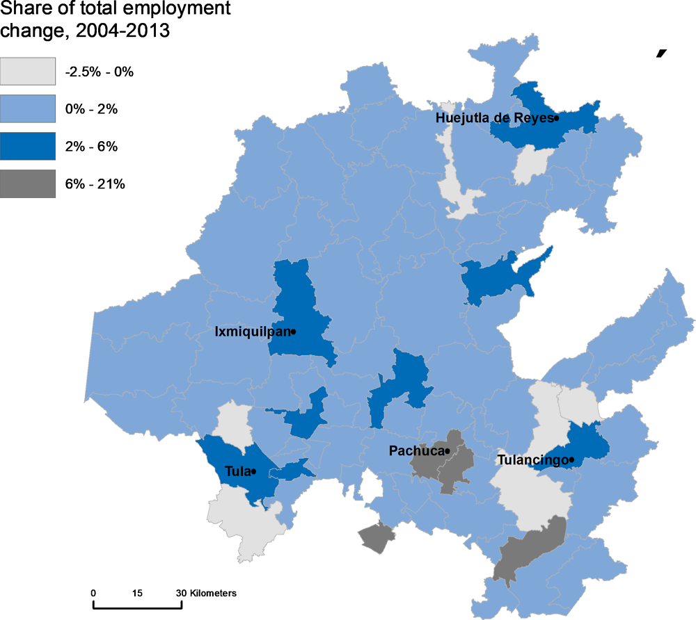
Source: INEGI (2015[19]), Economic census 2014.
Nevertheless, the contractual situation of formal workers in Hidalgo has become more precarious over time. Subcontracted employment has rapidly expanded, especially in services. About half of formal employees in 2013 were salaried workers, while 38% were business owners, family and non-salaried workers and 12% were workers without a contractual relationship (a category that captures outsourced employment) (Table 1.3). The share of outsourced employment increased 7 percentage points between 2004 and 2013, while the share of salaried workers decreased 8 percentage points over the same period.
Although outsourced employment is more commonly associated with the manufacturing sector (e.g. as part of processes involving maquiladoras), outsourcing levels and growth are larger in the service sector. In particular, one out of three formal workers in the wholesale and retail sector has a non-contractual relationship, which is significant given this sector employs one out of three workers in Hidalgo.
Note: Sectors with a share smaller than 2% not shown.
Source: INEGI (2015[19]), Economic census 2014.
Informality rates diminish slowly due to structural factors
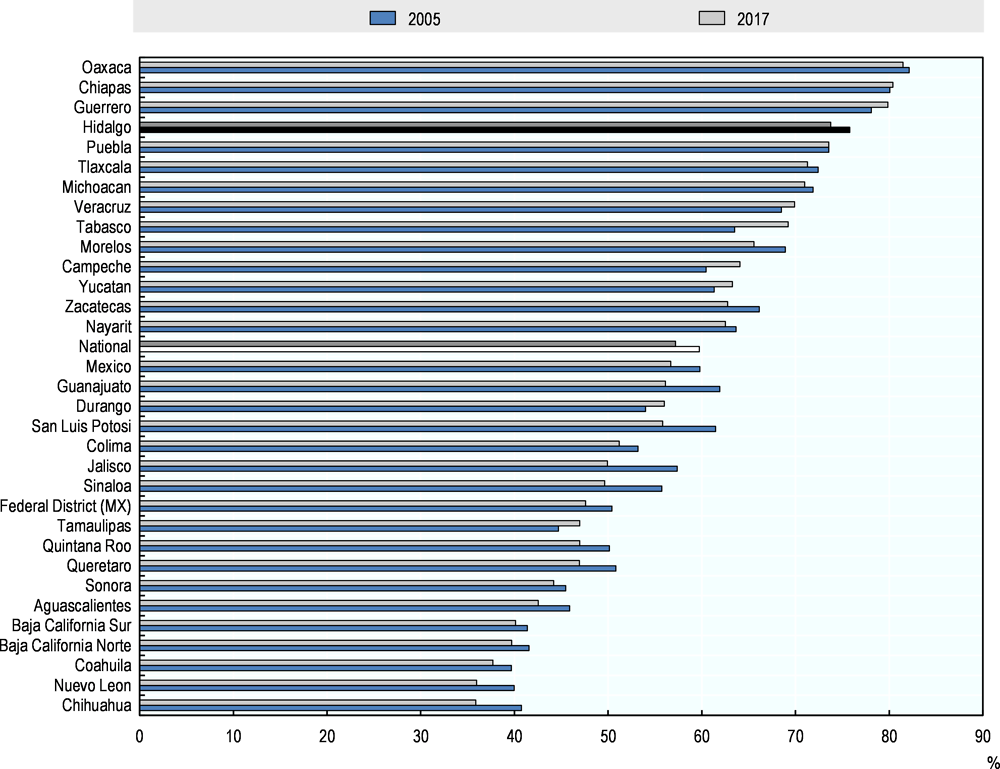
Labour informality in Hidalgo is high for national and Latin American standards and has not significantly decreased in the past decade. In 2017, about 8 out of 10 occupied persons in Hidalgo were informally employed (Figure 1.36). Hidalgo’s informality rate is the fourth largest in Mexico, surpassing the national mean by 16.6 percentage points (see Box 1.2 for more explanation on the concept and measurement of informality). The difference with the national average was virtually the same in 2005, indicating the lack of a strong movement from informal to formal employment in the past decade. Hidalgo’s informality rate is high for Latin American standards, as the average non-agricultural informality rate across Latin American countries stood at 47%, and it is as high as 70% in Bolivia, Honduras, Paraguay and Peru (International Labour Organization, 2016[24]).
The measurement and interpretation of informality in Mexico aligns with the International Labour Organization 2012 guidelines. According to these, informality in the productive sector has two dimensions. The first is related to the type or nature of the economic unit. Informal businesses are small, unregistered, home-based businesses producing legal goods and services that do not keep basic accounting records. Employment in informal businesses is catalogued as informal employment. The second relates directly to informal employment and includes individuals working outside the labour employment protection system of the country for formal or informal businesses.
Mexico uses an analytical tool called the Hussmann matrix that tabulates types of economic units versus the type of contractual relationship and informality status from the worker point of view. This type of classification seeks to encompass traditional informal occupations –,such as working for an informal business unit or being a domestic worker – with other types of informality that also imply more vulnerability and a lower level of social protection, such as working for a formal firm and the government under an arrangement that does not comply with national legislation.
The Hussmann matrix also allows obtaining suitable values for other indicators of informality used in the international context, such as the percentage of informal employment in non-agricultural activities, which would be the sum of workers in informal non-agricultural business units plus non-agricultural workers categorised as informal.
Source: INEGI (2014[25]), México: Nuevas estadísticas de informalidad laboral, (Accessed July 2018) http://www.beta.inegi.org.mx/proyectos/enchogares/regulares/enoe/
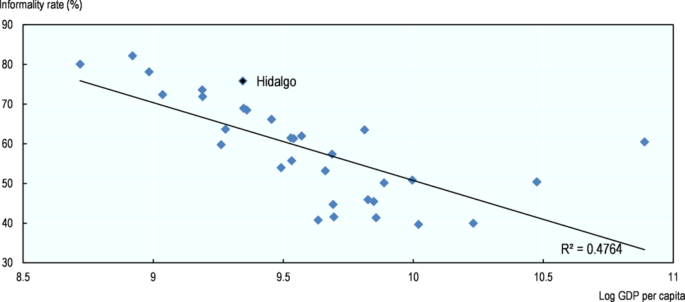
Informality levels in Hidalgo are larger than what income levels alone would predict. The correlation between informality rates and GDP per capita across Mexican states is -0.47, suggesting that states should witness decreases in informality rates as they develop (Figure 1.37). The informality rate in Hidalgo is larger than in four states with lower GDP per capita levels. This evidence suggests the existence of structural impediments to the mobilisation of informal workers and firms to the formal sector. These include a high share of microenterprises, the quality of human capital, restrictions on investment and businesses creation, and corruption levels (Dougherty and Escobar, 2013[26]).
Note: The informality rate is the total occupied workers with informal status over total occupied workers.
Source: INEGI (2017[27]), ENOE, III-Trimester 2017; INEGI (2005[28]) 2005-III trimester.
Across municipalities, higher GDP per capita, manufacturing shares and population density correlate with lower informality rates. The three factors can explain half of the variation in informality rates across 40 municipalities with available data (Table 1.4). Increases in population density and GDP per capita are related with similarly lower informality rates: in both cases, a 1% increase is associated with a decrease of 0.04 points in the informality rate. Moreover, more industrialised municipalities display on average lower informality rates: an increase of 1 percentage point of the manufacturing share is related to a decrease of 0.24 points in the informality rate.
Note: GDP per capita values expressed in natural logarithms.
Sources: OECD (2018[7]), Regional Economy, OECD Regional Statistics (database), https://doi.org/10.1787/a8f15243-en; INEGI (2017[27]), ENOE, III-Trimester 2017.
Across individuals, those younger, less educated and with larger families have a higher probability of being informally employed, and those with tertiary education living in richer municipalities have a lower probability. Having a level of schooling of primary education or less, the number of children and being younger than 25 years old all increase the probability of being informally employed, against the option of being formally employed (see Box 1.3 and Table 1.5 for details). On the other hand, having a tertiary or higher educational level and living in a municipality with a higher income per capita than the state means a decrease in the probability of being informally employed.
What kind of worker is more likely to be informally employed?
In a recent study for six Latin American countries, Fernández and co-authors propose a number of variables to explain the probability of being informally employed (as opposed to being formally employed) in each country. For Mexico, the results indicate that having a low level of education, being a married woman, being younger than 25 years old, residing in a rural area and the number of people living in the household are all significantly related to a higher probability of being informally employed. Being a female or being older than 55 do not significantly explain the probability of being informally employed. Fernández et al. also find that having tertiary education or more and residing in more productive cities is also related to a higher probability of being informally employed.
Performing a similar exercise for Hidalgo reveals some interesting results. In line with the national average, being younger than 25, having primary education or less and the size of the household are related with a higher probability of being informally employed. However, in Hidalgo, having tertiary education or more and living in a richer municipality reduces the probability of being informally employed, controlling for other factors (Table 1.5).
An informal worker in Hidalgo earns less than a formal worker with similar personal characteristics, occupation, sector of activity and place of residency. In 2017, the average hourly income from work for formal workers was 85% higher than that of informal workers. This difference reflects the fact that formal workers may be more educated, more experienced, work in better-paid occupations and/or work in sectors or live in municipalities that pay higher wages. However, calculating the income from work gap after controlling for all these and other factors, the formal-informal income from work gap between the two types of workers is still significant (Table 1.6). These results indicate that a formal worker earns 13% more per hour worked than a comparable informal worker. This gap can be interpreted as evidence of lower productivity in the informal sector and gives an idea of potential productivity gains from formalisation (Moreno Treviño, 2007[31]). Interestingly, the results on the determinants of income per hour worked also reveal that in Hidalgo a female worker earns 11% less than a comparable male worker.
A highly diverse informal sector calls for a set of complementary policies
The informal sector in Hidalgo is highly diverse in terms of profiles and economic sector. Roughly in line with national shares, three out of ten informal workers are own account workers while two in ten are subordinate workers in businesses, institutions and government (Table 1.7). Notably, the share of subordinate informal workers in primary activities is six percentage points higher in Hidalgo compared to the national average. In fact, the bulk of agricultural employment is informal, as the ratio of formal-to-informal workers in primary activities is above eight to one (Table 1.8). While most informal employment concentrates in service sectors, the share of informal employment in the manufacturing sector is almost ten percentage points lower than in the formal sector. The incidence of informality is far smaller in the manufacturing sector compared to the primary sector, as there are two formal manufacturing workers per every informal manufacturing worker.
Large informal sectors such as the one in Hidalgo are highly diverse in terms of worker profiles. In a typical region in Latin America, workers with extremely low levels of education and qualification earning only a fraction of the minimum wage can be found side by side highly educated workers earning more than the median formal wage (Günther and Launov, 2012[32]). Workers of different profiles have different reasons and motivations to be and stay informally employed. A key challenge for target policies is the difficulty in identifying the reasons behind informality, which include both observed (e.g. level of education) and unobserved characteristics (e.g. motivation and need for work flexibility).
The identification of segments within the informal sector can guide the design of targeted policies. One categorisation of informal employment identifies three types of informality based on the level of income and the educational level of workers (Fernandez et al., 2017[30]) (Figure 1.38). The first type is subsistence informality, grouping workers earning only a fraction of the minimum wage (bottom left quadrant in Figure 1.26). Subsistence workers typically have little demonstrable experience and low levels of productivity and are highly unlikely to transition to higher paying formal jobs and is at high risk of poverty and social exclusion. The second type, mixed informality, groups workers with low educational levels and comparable levels of income from work to formal workers. The third type is induced informality, comprising workers with low earnings and high educational levels. The explanation for the informal status in this group may be more related with personal or circumstantial reasons (e.g. difficult access to jobs, discrimination from employers based on personal characteristics or preference for flexible hours) than with productivity differences.
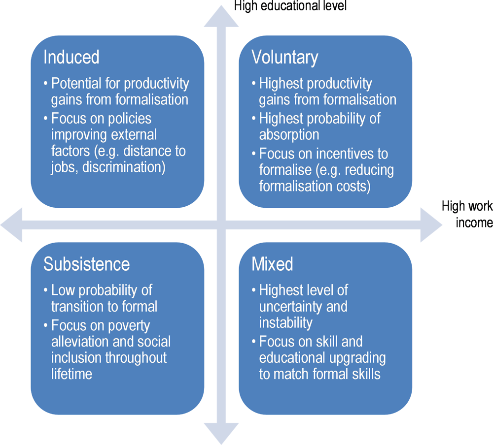
Source: Elaboration based on Fernandez et al (2017[30]), Taxonomía de la Informalidad en America Latina, http://www.repository.fedesarrollo.org.co/handle/11445/3476.
Most informal workers in Hidalgo face a high risk of poverty and exclusion. The split of individual informal workers by educational level and earnings reveals that one-third of informal workers belong to the “subsistence” category with average work earnings are less than half a minimum wage per month (Table 1.9). At the other end of the spectrum, about half belong to the “voluntary” or “induced” category as earnings per month are above one minimum wage per month. In terms of educational attainment, four in ten workers have completed up to primary school, and two in ten have completed tertiary education or higher levels. The subgroup of informal workers at the highest risk of poverty and exclusion which account for 16% of all informal workers (around 185 000 workers) comprises workers that have completed only primary education and earn half a minimum wage.
Workers in different informal categories are likely to respond differently to policies. Subsistence workers are unlikely to benefit from regulatory or institutional improvements leading to more formal job creation, as they would be likely outperformed when competing for low-skill formal jobs. This group is also at the highest risk of social exclusion because of their disadvantageous situation in the labour market and their low levels of income from work. Workers in the mixed category face a high risk of falling under the subsistence category, as their skill and educational levels make them relatively uncompetitive in the labour market. Workers in this group are likely to benefit from targeted skill upgrading and educational programmes that allow them to compete for formal jobs. Finally, workers in the induced/voluntary category could benefit from improvements in barriers to labour hiring, including excessive burdens on formal firms, as well as focal policies to bridge the spatial separation of low-income workers residencies and formal jobs. Given that workers in this group have relatively high levels of education and qualifications, their inclusion in the formal sector is likely to translate into productivity gains for the economy.
Reducing poverty, ensuring access and improving well-being
Lifting people out of poverty and deprivation is a pressing need
Most of the Hidalgo’s population needs to be lifted out of poverty and deprivation. Half of the state population is in poverty according to a multi-dimensional poverty rate that considers both income and deprivation in terms of access to education, health, housing, and food security. Hidalgo has the 9th largest poverty rate across 31 states and the former Federal District (now Mexico City) in Mexico. In 2016, Hidalgo had similar levels to Morelos and Tabasco.
Structural trends may be in favour of further poverty reduction in Hidalgo. Between 2014 and 2016, the state’s poverty rate decreased by around 4 percentage points. Currently, it is around six percentage points below the national average. Poverty rates are much higher in southern states of a comparable economic size such as Chiapas and Oaxaca. This geographical divide in poverty rates is likely to be persistent, as it is related to structural factors such as the difference in exposure to trade (Hanson, 2007[33]). Although Hidalgo has one of the highest poverty rates amongst states located in the north of Mexico, unlike southern states it is likely to benefit from structural trends in poverty reduction due to its geographic location.
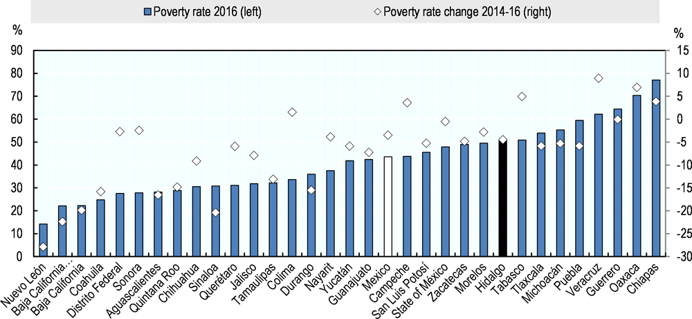
Note: Poverty rates weight income and level of deprivation in terms of education, health, housing and food security. Subsistence lines are set to MXN 1 857 in rural areas and MXN 2 858 in urban areas.
Source: CONEVAL (2017[34]), Poverty Measurement, https://www.coneval.org.mx/Medicion/Paginas/PobrezaInicio.aspx.
Extreme poverty in the state is located geographically in rural areas.2 Out of the population in poverty, 8% of the population (about 234 000 people) are in extreme poverty. On top of this group, 31.9% of the population with above subsistence income experience deprivation, leaving a minority of 12.8% of the population in a no poverty, no deprivation situation. The north concentrates the municipalities with the highest poverty rates (Figure 1.40). Extreme poverty in non-metropolitan areas stands at 13% of the population, far above the 3% in metropolitan areas. Some low densely populated municipalities in the north such as Tepehuacán de Guerrero, Xochiatipan and Yahualica have more than 80% of the population living in poverty, a child mortality rate of 20% and more than one-third of their population experience deprivation in terms of access to food.
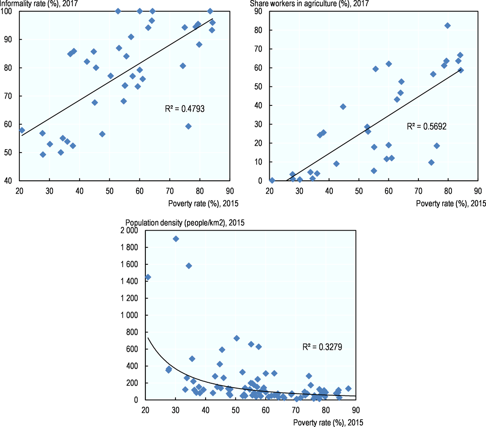
Whereas a successful transition away from agriculture and informality can lead to poverty reduction, poverty in low-density areas is likely to persist. Across municipalities in Hidalgo, poverty rates are higher in lower density municipalities with an agricultural vocation and higher informality rates (Figure 1.41). Remote places concentrate more poverty (compare Figure 1.15 and Figure 1.40). The structural change towards higher productivity activities has a potentially powerful impact on poverty through its positive effect on work incomes. However, areas with low accessibility, extremely high levels of informality and agricultural work will be the last to experience the benefits of this channel if they cannot accelerate the transformation of their productive bases. The existence of spatial poverty traps further affects the unequal effect of structural change on poverty reduction as they create vicious circles that exacerbate territorial inequalities (Bird, Higgins and Harris, 2010[35]).
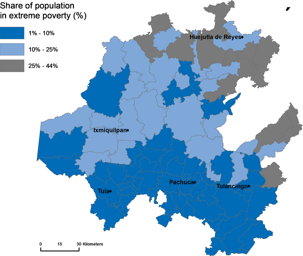
Note: Extreme poverty is based on CONEVAL definition: a person is in a situation of extreme poverty when he has three or more deficiencies, of six possible, within the Index of Social Deprivation and that, moreover, is below the minimum welfare line.
Source: Calculations based on CONEVAL (2015[36]), Poverty Measurement by Municipality, https://www.coneval.org.mx/Medicion/Paginas/PobrezaInicio.aspx.
Note: Poverty rates weight income and level of deprivation in terms of education, health, housing and food security. Subsistence lines are set to MXN 1 857 in rural areas and MXN 2 858 in urban areas.
Municipalities with higher informality rates, more workers in agriculture and lower density have higher poverty rates.
Source: INEGI (2017[27]), ENOE, III-trimester 2017; CONEVAL (2015[36]), Poverty Measurement by Municipality, https://www.coneval.org.mx/Medicion/Paginas/PobrezaInicio.aspx.
Improving well-being and equity requires ensuring proper access to basic services
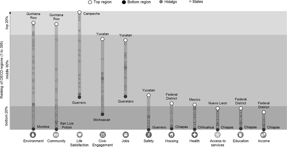
Recent economic gains have still to translate into improvements in well-being, especially with respect to life satisfaction and housing provision. Comparing regional well-being indicators across OECD regions (see Box 1.4) shows that Hidalgo’s rank in terms of the environment, life satisfaction, civic engagement and jobs is par with average performance across OECD regions (Figure 1.41). Similar regions in terms of well-being across OECD countries include Maule (Chile), East Macedonia–Thrace (Greece), Sicily (Italy) and North-Eastern Anatolia (Turkey).
Building comparable well-being indicators at a regional scale
The OECD framework for measuring regional well-being builds on the Better Life Initiative at the national level. It goes further to measure well-being in regions with the idea that measures at local level represent a more meaningful indicator. Besides place-based outcomes, it also focuses on individuals, since both dimensions influence people’s well-being and future opportunities.
In line with national well-being indicators, regional well-being indicators concentrate on informing about people’s lives rather than on means (inputs) or ends (outputs). In this way, the well-being features can be improved directly by policies. Regional well-being indicators also serve as a tool to evaluate how well-being differs across regions and groups of people.
Regional well-being indicators are multi-dimensional and include both material dimensions and quality of life aspects. Whenever possible, as in the case of Mexican states, self-reported experiences of well-being (subjective indicators) are also included. They also recognise the role of citizenship, institutions and governance in shaping policies and outcomes.
Although well-being dimensions are measured separately, the aim of the regional well-being framework is to allow for comparisons and interactions across multiple dimensions to account for complementarities and trade-offs faced by policymakers. At the same time, the comparison on regional well-being indicators over time allows comparing the dynamics of well-being over time, as well as the sustainability and resilience of regional development.
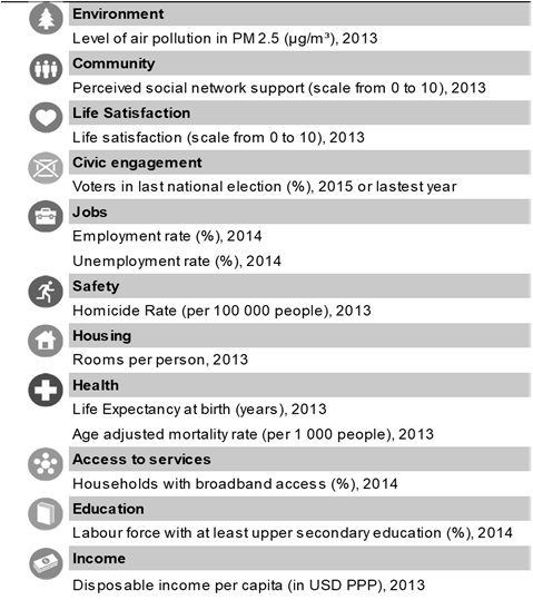
Regional well-being in Mexico is measured using 12 well-being dimensions: income, jobs, housing, health, access to services, education, civic engagement and governance, environment, life satisfaction, and safety – for which there are comparable statistics at the regional level – and three 3 dimensions: work-life balance, community (social connections) and life satisfaction – for which in the OECD database are available only at national level for lack of comparable data at the sub-national level. Table 1.10 details the indicator used for each dimension.
|
Table 1.10. Indicators by well-being dimension, Hidalgo
|
|---|
 |
|
Sources: OECD (2015[37]), Measuring Well-being in Mexican States, https://doi.org/10.1787/9789264246072-en; OECD (2014[38]), How’s Life in Your Region?, https://doi.org/10.1787/9789264217416-en; OECD (2018[39]), OECD Regional Well-Being Database, www.oecdregionalwellbeing.org. |
Across Mexican regions, Hidalgo is a top performer in safety and health indicators. However, the state performs worse than other states in terms of life satisfaction, housing, access to services and income indicators, indicating that there is room to further translate economic growth gains into higher well-being across social groups. It is worth noting that job performance here is measured by employment and unemployment rates that do not capture sub-employment and informal employment.
Note: OECD 34 weighted average.
Source: OECD (2018[39]), OECD Regional Well-Being Database, www.oecdregionalwellbeing.org.
Hidalgo ranks above the average of Mexican states in security. Hidalgo’s homicide rate in 2015 was 8 deaths by homicide per 1 000 inhabitants, less than half of the national average of 17 (Figure 1.43). Homicide rates in Hidalgo are at similar levels to neighbouring states of Querétaro and Tlaxcala, and are below those of Veracruz and Puebla, despite a worsening on this security indicator between 2010 and 2015. Hidalgo ranks fourth across Mexican states in terms of security perception (Figure 1.44). In 2017, 43.3% of the population older than 15 years old declared they felt safe in the state, a similar share than in 2011.
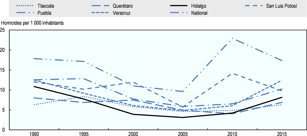
Sources: INEGI (2018[40]), Mortality: Deaths by Homicide, http://www.inegi.org.mx/sistemas/olap/proyectos/bd/continuas/mortalidad/defuncioneshom.asp?s=est; INEGI (2018[41]), Population by Federative Units, http://www.beta.inegi.org.mx/temas/estructura

Note: Higher values indicate a higher share of the state population older than 15 years who feel safe.
Source: INEGI (2018[42]), National Survey of Victimization and Perception of Public Safety (ENVIPE) 2017.
Large inequalities in access to health services imply that a significant share of the population does not have proper access to health services. Hidalgo has one of the lowest mortality rates across Mexican states, and a life expectancy of 74.3 years, 2 years less than the maximum of 76 years across Mexican states. However, these indicators do not fully reflect inequalities in access and provision. While 82% of the population of the state is affiliated to the health system (the bulk of which is public), this percentage can be as low as 30% across municipalities (INEGI, 2017[43]). Across the territory, while 18% of the population does not have access to a hospital within a 1-hour drive, 8.3% can access up to 4 hospitals within the same time (Table 1.11). Access to health facilities is even limited for the more numerous health centres scattered across the state for a portion of the population living in remote areas. In total, 20 606, 34 251 and 53 263 people do not have access to a health facility within a 30-, 45- and 60-minute car journey.
Inequalities in access to education reinforce the effect of inequalities in access to economic opportunities and lead to widening regional gaps. A significant share of young people in Hidalgo has restricted access to educational opportunities (Figure 1.45). Young people in some localities in northern regions cannot access any school within a 1-hour drive, while young people in localities with high access can access up to 148 secondary schools within a 1-hour drive. Young people in localities with low accessibility are likely to relocate in search for schooling opportunities or drop the schooling system altogether. In either case, the effect of such restricted access to schooling is an increase in regional disparities, as localities with low access are drained from young educated workers.
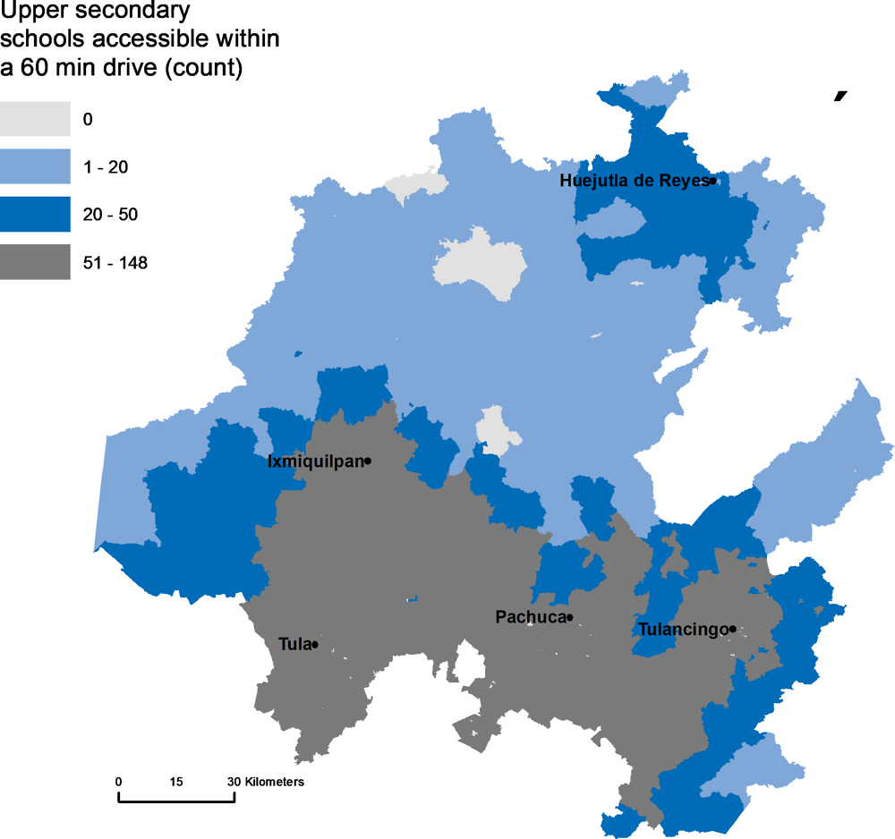
Note: Units represent the total number of schools accessible within a 60-minute drive threshold.
Within a 60-minute drive through the existing road network.
Sources: SEP (n.d.[44]), Sistema Nacional de Información de Escuelas, http://www.snie.sep.gob.mx/SNIESC/; Open Street Maps (2018[18]), database (accessed July 2018) https://www.openstreetmap.org INEGI (n.d.[17]), Conjunto de Datos Vectoriales de Carreteras y Vialidades Urbanas Edición 1.0 (Distribución por Entidad Federativa), http://www.inegi.org.mx/geo/contenidos/topografia/vectoriales_carreteras.aspx.
Closing physical access gaps with remote access in Hidalgo will require substantial expansion of the information and communications technology (ICT) infrastructure. In 2017, 67% of households in Hidalgo lacked an Internet connection, a higher percentage than the national average of 49.1% and far above the share of Mexico City where only one-quarter of households lack an Internet connection (INEGI, 2017[45]). On the same year, about six out of ten households in reported not having a computer at home. Ensuring wider Internet coverage through investments across the territory presents opportunities for the next generation, as young people represent a larger share of Internet users than across the average of states in Mexico – the share computer users in the 6-17 age range is 41%, 7 percentage points higher larger than national mean of 34.1%.
Concluding remarks
The evidence reviewed in this chapter suggests that in Hidalgo there is room for productivity improvements. These improvements can stem from structural change away from low productivity services and towards higher value-added, higher productivity tradable services, such as the information related activities. Hidalgo needs to diversify its economic structure towards less volatile sectors in the near future. Further analysis of the specialisation patterns and trends in the manufacturing sector can help understanding if future expansions of the manufacturing sector in Hidalgo will effectively translate into more manufacturing jobs with at least the same intensity.
The assessment of this chapter indicates the need for urgent and aggressive innovation policy action to tackle the increasing technological gap and pave the way for a transition to higher technology sectors. Furthermore, improving conditions in the labour market will require the design of tailored incentives for informal workers of different socio-economic profiles.
References
[5] Banxico (2018), Balanza Comercial, http://www.banxico.org.mx/SieInternet/consultarDirectorioInternetAction.do?accion=consultarCuadro&idCuadro=CE125§or=1&locale=es.
[4] Banxico (2018), Índice del Tipo Real de Tasa de Cambio, http://www.banxico.org.mx/SieInternet/consultarDirectorioInternetAction.do?sector=6&accion=consultarCuadro&idCuadro=CR60&locale=es.
[35] Bird, K., K. Higgins and D. Harris (2010), “Spatial poverty traps: An overview”, No. 161, Overseas Development Institute, http://www.odi.org.ukiiAcknowledgements (accessed on 22 August 2018).
[8] Brezzi, M., L. Dijkstra and V. Ruiz (2011), OECD Extended Regional Typology: The Economic Performance of Remote Rural Regions, OECD Publishing, Paris, https://doi.org/10.1787/5kg6z83tw7f4-en.
[34] CONEVAL (2017), Poverty Measurement, https://www.coneval.org.mx/Medicion/Paginas/PobrezaInicio.aspx.
[36] CONEVAL (2015), Poverty Measurement by Municipality, https://www.coneval.org.mx/Medicion/Paginas/PobrezaInicio.aspx.
[10] CONEVAL (2010), Multidimensional measurment of poverty.
[26] Dougherty, S. and O. Escobar (2013), “The Determinants of Informality in Mexico's States”, OECD Economics Department Working Papers, 2013/1043, No. 1043, OECD Publishing, Paris, https://doi.org/10.1787/5k483jrvnjq2-en.
[30] Fernandez, C. et al. (2017), “Taxonomía de la informalidad en America Latina”, Fedesarrollo, http://www.repository.fedesarrollo.org.co/handle/11445/3476.
[21] German-Soto Vicente (2017), Generación del Producto Interno Bruto Mexicano por Entidad Federativa, 1940-1992.
[46] Geurs, K. and B. van Wee (2004), “Accessibility evaluation of land-use and transport strategies: review and research directions”, Journal of Transport Geography, Vol. 12/2, pp. 127-140, https://doi.org/10.1016/j.jtrangeo.2003.10.005.
[32] Günther, I. and A. Launov (2012), “Informal employment in developing countries”, Journal of Development Economics, Vol. 97/1, pp. 88-98, https://doi.org/10.1016/j.jdeveco.2011.01.001.
[33] Hanson, G. (2007), “Globalization, labor income, and poverty in Mexico”, in Globalization and Poverty, University of Chicago Press.
[29] INEGI (2018), Censo Económico 2015.
[40] INEGI (2018), Mortality: Deaths by Homicide, http://www.inegi.org.mx/sistemas/olap/proyectos/bd/continuas/mortalidad/defuncioneshom.asp?s=est.
[42] INEGI (2018), National Survey of Victimization and Perception of Public Safety (ENVIPE) 2017.
[41] INEGI (2018), Population by Federative Units, http://www.beta.inegi.org.mx/temas/estructura/.
[43] INEGI (2017), Anuario estadístico y geográfico de Hidalgo 2017.
[20] INEGI (2017), Directorio Estadístico Nacional de Unidades Económicas (database).
[14] INEGI (2017), Encuesta Inter-censal 2015.
[27] INEGI (2017), ENOE, III-Trimester 2017.
[45] INEGI (2017), INEGI. Encuesta Nacional sobre Disponibilidad y Uso de TIC en Hogares, ENDUTIH 2017.
[6] INEGI (2017), Marco Geoestadístico Nacional, http://www.beta.inegi.org.mx/temas/mapas/mg/.
[19] INEGI (2015), Economic census 2014.
[25] INEGI (2014), México: Nuevas estadísticas de informalidad laboral, http://www.beta.inegi.org.mx/contenidos/proyectos/enchogares/regulares/enoe/doc/Informalidad_final.pptx (accessed July 2018).
[15] INEGI (2013), Continuo de Elevaciones Mexicano (CEM 3.0), http://www.beta.inegi.org.mx/app/geo2/elevacionesmex/ (accessed July 2018).
[13] INEGI (2010), Censo Poblacional 2010.
[9] INEGI (2010), Cuentame INEGI, http://www.cuentame.inegi.org.mx/monografias/informacion/hgo/poblacion/m_migratorios.aspx?tema=me&e=13.
[28] INEGI (2005), 2005-III trimester.
[17] INEGI (n.d.), Conjunto de Datos Vectoriales de Carreteras y Vialidades Urbanas Edición 1.0 (Distribución por Entidad Federativa), http://www.inegi.org.mx/geo/contenidos/topografia/vectoriales_carreteras.aspx.
[24] International Labour Organization (2016), 2016 Labour Overview: Latin America and the Caribbean.
[23] Jütting, J. and J. de Laiglesia (2009), Is Informal Normal?: Towards More and Better Jobs in Developing Countries, Development Centre Studies, OECD Publishing, Paris, https://doi.org/10.1787/9789264059245-en.
[31] Moreno Treviño, J. (2007), “Los salarios del sector formal e informal en México: Análisis de ganancias y pérdidas por formalización”, Ensayos Revista de Economía, Vol. 26/1, pp. 1-44, http://eprints.uanl.mx/7815/ (accessed on 17 August 2018).
[22] National Registry of Foreign Investment (2018), National Registry of Foreign Investment, Secretary of Economy, https://www.gob.mx/se/acciones-y-programas/competiti.
[1] OECD (2018), Economic Outlook 103 - May 2018, https://stats.oecd.org/index.aspx?DataSetCode=EO.
[39] OECD (2018), OECD Regional Well-Being Database, http://www.oecdregionalwellbeing.org.
[7] OECD (2018), Regional Economy, OECD Regional Statistics (database), https://doi.org/10.1787/a8f15243-en.
[11] OECD (2017), Building an Inclusive Mexico: Policies and Good Governance for Gender Equality, OECD Publishing, Paris, https://doi.org/10.1787/9789264265493-en.
[2] OECD (2017), OECD Economic Surveys: Mexico 2017, OECD Publishing, Paris, https://doi.org/10.1787/eco_surveys-mex-2017-en.
[37] OECD (2015), Measuring Well-being in Mexican States, OECD Publishing, Paris, https://doi.org/10.1787/9789264246072-en.
[38] OECD (2014), How's Life in Your Region?: Measuring Regional and Local Well-being for Policy Making, OECD Publishing, Paris, https://doi.org/10.1787/9789264217416-en.
[12] OECD (2014), PISA 2012 Results: What Students Know and Can Do (Volume I, Revised edition, February 2014): Student Performance in Mathematics, Reading and Science, PISA, OECD Publishing, Paris, https://doi.org/10.1787/9789264208780-en.
[3] OECD Statistics (2018), Inflation (CPI), https://data.oecd.org/price/inflation-cpi.htm.
[18] OpenStreetMaps (2018), Database, http://www.openstreetmap.org (accessed on 2018).
[44] SEP (n.d.), Sistema Nacional de Información de Escuelas, http://www.snie.sep.gob.mx/SNIESC/.
[16] Weiss, D. et al. (2018), “A global map of travel time to cities to assess inequalities in accessibility in 2015”, Nature, Vol. 553, p. 333, https://doi.org/10.1038/nature25181.
In an increasingly globalised economy, regions with similar initial levels of economic development and economic size face similar capacity restrictions in terms of economies of scale and productive capacity.
In this context, the share of manufacturing is indicative of the relative importance of tradable goods and the exposure of the region to international changes in the demand for manufactures. Evaluating the performance of Hidalgo over time with respect to regions that had similar initial levels is therefore indicative of the relative performance of the region in the global arena.
Following this, the selection of a group of comparable regions across more than 700 OECD regions is based on similarity in 3 criteria: i) initial economic development, as measured by GDP per capita in 2003; ii) initial market size, as measured by total population in 2003; and iii) initial relative importance of manufacturing, as measured by the share of GVA in manufacturing in 2004. The range to establish similarity was set to between half and double of Hidalgo’s 2003 values.
Annex Table 1.A shows the resulting group of comparable regions, excluding two regions in Brazil for which there was no information available on employment and GVA. The group include the Central Mexican regions of Querétaro and Morelos, which share with Hidalgo the proximity to the Mexico State and Federal District, as well as six other Mexican regions of similar size and manufacturing vocation. Across other OECD countries, the comparable regions include 13 regions located in East European countries and a Baltic region involved in Global Value Chains in manufacturing.
Accessibility can be defined as the easiness with which people in different locations can physically access markets, for goods, services and employment and business opportunities (Geurs and van Wee, 2004[46]). Access to cities is the time (in minutes) it takes to reach a city of at least 50 000 inhabitants. At the level of municipality, access to a city refers to the median time needed to reach the closest city (within or outside the state borders) calculated from 1 km2 impedance values. A city is defined as “contiguous cells with a density of at least 1 500 per km2 or a density built up greater than 50% and a minimum population of 50 000 inhabitants” (Weiss et al., 2018[16]). The impedance travel grid summarises the availability of roads, railroads, waterways and topographical conditions. Journey times summarise how long it takes to reach a location using the most efficient route and the fastest mode available at every grid cell. For more details on the impedance grid see Weiss et al (2018[16]).
Another common measure of accessibility is the cumulative opportunity (CO) index, which measures how many opportunities (people, schools, hospitals, etc.) can be reached under a certain commute threshold using a certain transportation mode. Ideally, accessibility should consider all transportation modes, especially where a large percentage of the population does not have access to a vehicle. However, comprehensive public transport information is not available for the case of Hidalgo. In the CO index, the estimated travel times between each locality (localidad) refer to shortest-path travel times by car using the existing road network.
Three measures of “opportunity” by locality are defined based on the Origin-Destination matrix with travel times between localities in Hidalgo. The first is the number of people, which also includes localities in the southern edge of Hidalgo. The measure of accessibility to people is then the percentage of the total population accessible in reachable localities in Hidalgo, the state of Mexico and Mexico City. The second opportunity measure is the number of upper secondary schools aggregated by locality from precise point-co-ordinates. The third opportunity is health facilities, split between hospitals and health centres, also summed by locality from precise point co-ordinates.
The last step involves calculating the index for commuting times below a 60-minute threshold. For every locality Y, the CO index answers the question: how many opportunities can a person reach after commuting by car for 60 minutes from locality Y in every possible direction using the existing road network?
Notes
← 1. The index of Geographic Concentration of population or businesses is defined as: , where is the population/businesses share of municipality i, is the area share of municipality i.
← 2. According to CONEVAL, a person in extreme poverty is when he does not meet three or more indicators, of six possible, within the Social Deprivation Index and which, moreover, is below the minimum welfare line. People in this situation have such a low income that, even if they dedicate it completely to the acquisition of food, they could not acquire the necessary nutrients to have a healthy life.