Chapter 5. Criteria to guide nitrogen policy making
This chapter provides a framework for analysing the merits of nitrogen management policy instruments. It establishes a typology of the different types of instruments available to decision makers and proposes three criteria to evaluate them (effectiveness, cost-efficiency and feasibility). It stresses the importance of strengthening the coherence between nitrogen pollution management policy and other policies, both environmental and sectoral.
Whatever the policy approach is (risk or precautionary), evaluation criteria are needed to select the right risk management or uncertainty management tools (Figure 5.1). Firstly, it is necessary to evaluate and address the unintended effects on nitrogen of sectoral (e.g. agricultural policy, energy policy) and environmental policies (climate policy and others). Nitrogen policy instruments that are cost-effective and whose "feasibility" of implementation is not problematic may then be selected. Finally, due to the nitrogen cascade, the unintended effects of an instrument targeting one form of nitrogen on other forms of nitrogen should be estimated, in order to promote synergies and avoid “pollution swapping”.
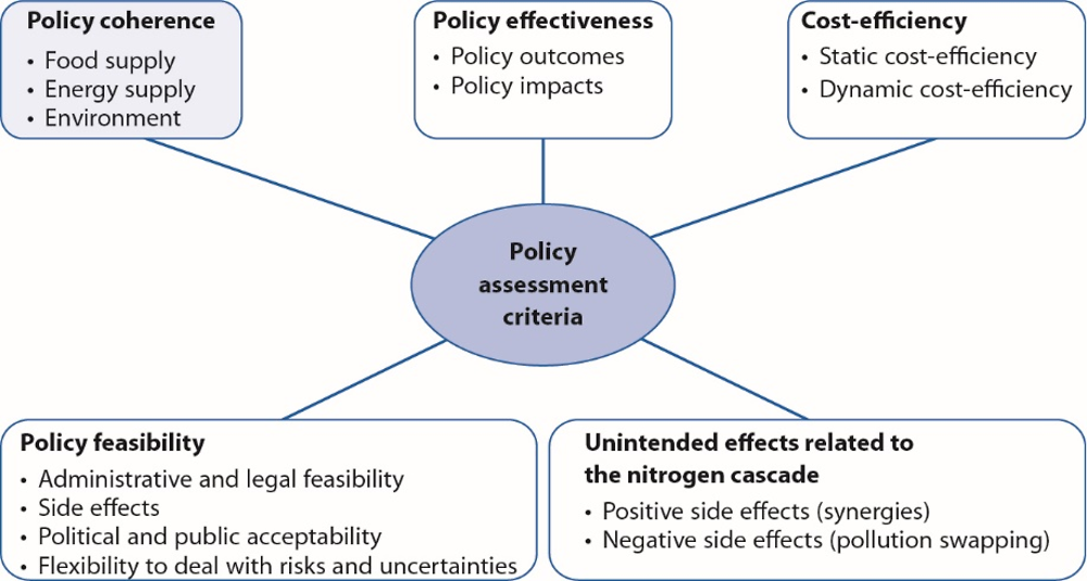
Note: The policy coherence criteria applies to policies not primarily focused on the management of nitrogen pollution.
Source: Adapted from Drummond et al. (2015).
An example of what the search for consistency with agricultural policy may involve is given in Section 5.1 below.1 Section 5.2 introduces the criteria of effectiveness, cost-efficiency and feasibility for designing nitrogen policy instruments. Applying these criteria to different types of policy instruments, Chapter 6 presents their advantages and disadvantages, in a generic sense, as well as case studies on nitrogen policy instruments. The assessment of the unintended effects of the nitrogen cascade is just beginning (see Section 5.3); Chapter 4. presented a case study on agricultural practices.
5.1 Policy coherence
First and foremost, it must be ensured that sectoral policies do not encourage excessive nitrogen production. This may be the case with some policies aimed at stimulating agricultural production or the security of energy supply.
For example, Bartelings et al., 2016 estimated the impact of subsidies on fertiliser production and use on greenhouse gas (GHG) emissions using a computable general equilibrium model.2 First, ad-valorem subsidy rates were calculated from information on fertiliser costs. For example, Indonesia and India have a policy of reducing energy costs in fertiliser production in order to provide fertiliser to national farmers at a lower cost.3 It is estimated that the resulting public financial support reduces the cost of nitrogen fertiliser for Indonesian farmers by 68% below production costs and by 56% for Indian farmers (Table 5.1). Russia and China support fertiliser use through direct subsidies to farmers. It is estimated that the input subsidy (implemented as an area payment in China) is equivalent to an ad valorem subsidy of about 28% of the value of fertiliser cost in Russia, and 12.5% in China (Table 5.1).
Second, GHG emissions in relation to fertiliser production and use were estimated (Table 5.2). This is obviously an approximation since nitrous oxide (N2O) emissions from crops depend on farming practices and not just on fertilisation rates. In particular, the application of the 4R concept (the right type of fertiliser at the right rate applied at the right time in the right place)4 can both increase the efficiency of nitrogen uptake by plants and reduce excess nitrogen in the field, thus reducing N2O emissions (Omonode et al., 2017).
GHG emissions of crops also depend on the type of fertiliser (with N2O emissions typically being higher for urea than for ammonium nitrate) and soil type, with N2O emissions generally high for clay soils with poor drainage (Figure 5.2). Previous internationally accepted estimates were that for every kg of nitrogen fertiliser applied in grain crop production, there is a loss of 1% as N2O to the atmosphere. 5
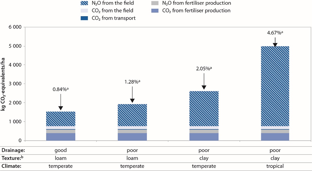
a. Nitrous oxide (N2O) emissions from the field as a % of applied nitrogen fertiliser; calculated according to the Bouwman model (Bouwman et al., 2002) with an uncertainty range of -40% to + 70%.
b. Other important soil factors are soil organic carbon and pH.
Source: Brentrup and Pallière (2009).
Finally, the GHG emission reduction impact of phasing out fertiliser subsidies was estimated. The impact differs by country. It is particularly pronounced in India and Indonesia where, with the elimination of subsidies paid directly to the fertiliser industry, locally produced nitrogen would become less attractive than imported phosphorus and potassium (substitution effect between the three nutrients). The model shows that GHG emissions would also decrease in China, where the removal of input-related area payments (linked to both land and fertiliser use) would lead to a reduction in agricultural production. While GHG emissions from nitrogen use would fall in Russia, emissions from fertiliser production would rise as Russia would begin to export nitrogen to India and Indonesia.
According to the study, the abolition of fertiliser subsidies would only have a modest effect on agricultural land use in all four countries, except for China. In China, the phasing out of fertiliser subsidies could lead to an increase in carbon sinks, as forests could develop on land that is no longer used for agricultural purposes, adding to the net reduction of GHG emissions.
In fact, China has taken steps to phase out fertiliser subsidies and aims to cap fertiliser use by 2020. The 2020 Zero-Growth Action Plan for Chemical Fertilisers and Pesticides aims to reduce the annual growth of chemical fertiliser use to below 1% for the 2015-19 period and achieve zero-growth by 2020 for major agricultural crops (OECD, 2016b). However, these policy developments need to be assessed in a context of increasing policy support for Chinese farmers, largely through forms of support that distort agricultural production (Figure 5.3).

Source: OECD (2018a).
To sum up, some forms of agricultural support can distort input use and agricultural production and thus have negative environmental impacts (such as increased emissions of N2O). Before designing targeted policies on nitrogen pollution, it is therefore essential to monitor and evaluate sectoral policies and their unwanted effects on nitrogen emissions. The OECD has established a typology of support measures for agricultural producers and is working on an assessment of their environmental impact (see for example OECD, 2018b). The OECD has also developed expertise in the monitoring and evaluation of policies that directly support the production or consumption of fossil fuels. This OECD work could provide a basis for assessing the adverse effects of sectoral policies on nitrogen pollutant emissions.
Policy coherence must also be sought with environmental policies that are not primarily aimed at reducing nitrogen pollution. For example, in New Zealand, a policy to reduce carbon dioxide (CO2) emissions has helped reduce the leaching of nitrate (NO3-) into water (in part, following OECD, 2013). A GHG Emissions Trading Scheme (ETS) allows GHG emitters who do not want to reduce their emissions to enter into agreements (through a Trust) with farmers who agree to sequester carbon. With financial compensation, farmers undertake to convert pastoral lands into forests, thereby helping to reduce the leaching of NO3- into water. GHG emitters receive ETS credits in exchange for pastoral land converted to forestry (Figure 5.4).
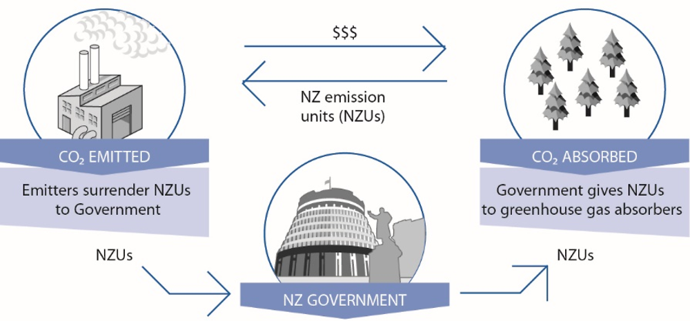
Source: Ministry for the Environment of New Zealand, www.mfe.govt.nz/climate-change/reducing-greenhouse-gas-emissions/about-nz-emissions-trading-scheme, accessed 29 March 2018.
This is occurring in Lake Taupo, the largest lake in the country, which is threatened by nitrogen pollution. To reduce nitrogen pollution in the lake, a cap-and-trade system for nitrogen was put in place for farmers around Lake Taupo. Instead of selling their nitrogen pollution rights, farmers can opt for permanent reductions in nitrogen, for which they are compensated financially through the Trust. In turn, the Trust is funded by GHG emitters through the purchase of ETS credits. Farmers are paid for the reduction of nitrogen emissions, at the same time they receive income from forest credits.
This example of environmental measures not focusing on nitrogen pollution but helping to manage it explains why coherence must also be sought in environmental policies. As a counterexample, assessing trade-offs between climate change mitigation goals and nitrogen pollution management may be more challenging when it comes to forest fertilisation,6 which increases both the sequestration of carbon and the risks associated with nitrogen. According to de Vries, 2017 nitrogen deposition has contributed to a significant increase in carbon sequestration in forests and forest soils in Europe since 1950. However, nitrogen aerosol deposition may also contribute to decreasing the drought tolerance of forest trees by decreasing the opening of stomata7 in their leaves (Burkhardt and S.Pariyar, 2014; Grantz et al., 2018).
5.2 The effectiveness, efficiency and feasibility of policy instruments8
5.2.1 A typology of policy instruments
Policy instruments of extremely varied design and practical application may be employed for the control of nitrogen pollution. Based on the classifications provided by OECD (2008), such instruments may be placed into the following categories:
-
Pricing instruments: environmentally related taxes and charges and tradable permit systems (TPS)
-
Direct environmental regulation (DER)
-
Financial support instruments: public financial support (PFS) and payments for ecosystem services (PES)
-
Information measures
-
Voluntary schemes
Environmentally related taxes are compulsory duties levied by a competent authority (either a national, regional or local government) on legal entities concerning certain products, activities or transactions with the aim of discouraging environmentally harmful behaviour through price disincentives. Environmental charges are payments made by consumers to providers of environmental management services, such as wastewater treatment.
The TPS are quantity-based instruments that assign property rights to units of positive or negative (actual or potential) externalities (such as pollutants or ecosystem services), which after allocation may be traded as a commodity between obligated entities on newly-created markets. The most common design is a ‘cap-and-trade’ approach, in which an aggregate cap on the volume of a pollutant is set (below that which would be produced in absence of a cap) and permits assigned for each unit of pollutant under the cap, affording the bearer a ‘right’ to emit or discharge a unit of pollutant, creating scarcity and a market value. ‘Baseline and credit’ systems, rather than setting a cap with a finite number of tradable permits, create and award credits (permits) to entities that reduce pollution levels below a projected baseline, which may then be traded as above (with an aggregate cap retained and set by the projected baseline). A similar approach may be taken concerning ecosystem services i.e. credits issued for protecting or restoring ecosystem services, which may be traded to other entities to offset an increase in the need for such services – for example, reforestation to increase CO2 sequestration to offset increasing CO2 emissions; or creating wetlands to maximize denitrification in NO3- enriched watersheds (Hansen et al., 2016).
DER refer to the imposition of minimum or maximum standards, limits or bans on, or requirements for, certain products, practices or performance levels (such as ‘Best Available Technologies’ (BAT)), and other similar obligations, such as activity permits.
PFS refers to the use of the public budget to encourage practices with reduced environmental impact (or discourage those with high impact), to foster organisational or technological innovation, or to finance infrastructure. Such support may be given via numerous channels, including direct budget allocations or grants, low or zero interest loans, loan guarantees, or preferential tax treatment (OECD, 2008).
Various definitions of the PES concept exist, with no agreed single definition (Schomers and Matzdorf, 2013). However, PES may be broadly defined as a transaction where ecosystem managers (e.g. land owners) are compensated through conditional payments by the beneficiaries of ecosystem services (including governments, where the public is the general beneficiary) for the additional cost of maintaining ecosystem services above legally required levels.
Information measures attempt to overcome information failures through awareness campaigns, labelling and certification schemes, training and education programmes, the provision of ‘best practice’ guidelines, and disclosure and reporting mechanisms.
Voluntary schemes include environmental management systems, voluntary agreements negotiated between government and certain economic sectors, unilateral sectoral or cross-sectoral agreements to achieve a given environmental objective.
No single instrument or type of instrument is appropriate for tackling all sources of pollution, from all sectors. Whilst this section introduces types of policy instruments individually, it will probably be desirable to introduce instruments in combination, as a policy ‘mix’. Both individual instruments and policy mixes experience trade-offs between the three assessment criteria discussed below. Such trade-offs are unavoidable in a ‘second-best’ world, characterised by multiple market failures and uncertainties.
5.2.2 Effectiveness, efficiency and feasibility criteria
Existing policy analysis methodologies tend to assess the performance of a policy instrument against the criteria of economic efficiency – particularly static efficiency (i.e. the most productive balance between resource allocation and outcome, or when a desired outcome is given, achievement of this outcome at the lowest cost at a given point in time (static cost-efficiency)). Such analyses often recommend the use of pricing tools as cost-minimising solutions to reduce the emission of pollutants, particularly those encompassing all (anthropogenic) sources of the pollutant, over the full geographic scope in question. However, such a view neglects ‘real world’ complications that often act to limit policy effectiveness and the ability to introduce instruments in the more theoretically desirable manner. Such factors include (Görlach, 2013).
-
Market failures aside from the externality of the pollutant in question. Examples are information failures and principal-agent problems (split incentives), along with ‘satisficing’ behaviour,9 which can act to prevent the market from producing an ‘optimal’ outcome.
-
The development of abatement options. This may be stimulated to some extent by pricing policies, however such development is uncertain, and a high price may be required to stimulate private investment in the development of such technologies and practices.
-
Administrative feasibility, including pollutant and compliance monitoring, and enforcement. For some sources of pollution it may not be possible, or prohibitively expensive, to administer certain instruments. Any efficiency gain associated with a pricing instrument may be more than offset by the transaction costs of administration, monitoring and ensuring compliance for such sources.
-
Lack of public and political acceptability, which, along with legal compatibility, may prevent an otherwise suitable instrument from being introduced.
-
Distributional impacts and equity issues, which may also prevent an instrument’s introduction if they cannot be adequately addressed.
-
The global nature of some pollutants, such as GHGs. Policy instruments that simply shift such pollution to another jurisdiction rather than producing global abatement cannot be considered truly effective.
Such conditions suggest that broader policy assessment criteria are required to capture these nuances, and allow for a more rounded evaluation of the relative desirability of policy instruments for different applications.
‘Effectiveness’ concerns the results of a policy intervention, which may be defined in terms of policy outcomes (e.g. the use of catalytic converters in vehicles) or policy impacts (e.g. reduced disturbance of the nitrogen cycle). Which of these is applicable depends on the specific objectives of a given policy instrument, and of the assessment being carried out. For example, whilst the ultimate objective for instruments aiming to control nitrogen pollution is reduced disturbance of the natural nitrogen cycle, it may be impractical to ascribe such an impact to a single policy intervention. In such cases, policy objectives (if made explicit) are often defined in terms of a policy ‘outcome’ (Görlach, 2013).
Broadly, the ‘cost-efficiency’ criterion relates the inputs (costs) to the results (outcome/impact) of a policy intervention, and asks whether the intervention’s objective is being achieved at the least cost to society. This is composed of two sub-criteria. The first is static cost-efficiency, which requires all targeted sources of a given pollutant to face the same marginal abatement cost, and therefore equal incentive for abatement, so that any level of abatement from these sources is reached at the lowest cost for society as a whole, using the abatement options available at a given point in time. This is sometimes referred to as the equi-marginal principle. The second sub-criterion is dynamic cost-efficiency, which refers to achieving pollution abatement at the lowest possible societal cost over a given time period, by providing a continuous incentive to innovate and implement ever-cheaper abatement options (Duval, 2008). As such, dynamic cost-efficiency assumes temporally flexible rather than fixed abatement options and costs. From this perspective, encouraging the deployment of a currently expensive abatement technology to enable innovation and produce low-cost abatement for the future, in contrast to a static perspective, may be preferable to a lower cost-alternative with less potential for long-term cost-reduction (Görlach, 2013).
Pricing instruments are statically cost-efficient if the explicit or implicit price is applicable to and equalised across all sources of pollution within the scope of the instrument. A tax or TPS may have a broad geographical and sectoral scope, and may cover multiple fungible ‘commodities’ (pollutants). For example, pollutants that have the same (or comparable) impact, such as the production of eutrophication of water bodies by nitrogen and phosphorus. Pollutants that have different but stable levels of impact in relation to each other, such as GHGs with different global warming potentials (GWP), may also be considered in a single tradable permit system. For example, the number of permits required for the emission of a unit of a GHG with a high GWP may increase in proportion to the number of permits required for the emissions of a unit of a GHG with the lowest GWP within the scope of the instrument.
The ‘feasibility’ of instrument implementation is obviously essential if an instrument is actually to be introduced and function effectively. The concept may be broken down into five general aspects. The first is administrative feasibility, including, for example, the ease of administration, transaction costs and stringency of the compliance regime. The second concerns the ability to address side effects, intended and unintended, positive and negative. This may include negative distributional/equity impacts and impacts on industrial competitiveness, but also job creation, resource security and health and environmental co-benefits (Box 5.1). Linked to these two aspects are political and public acceptability, which are themselves clearly linked. The fourth aspect is legal and institutional feasibility, which considers the compatibility of a policy instrument with existing legal frameworks and constitutional doctrines. The final aspect concerns the flexibility of an instrument, and its ability to respond to new information and deal with risks and uncertainties. This also reflects the ability of an instrument to deal with strategic behaviour (either induced by asymmetric information, rent-seeking, regulatory capture, or even fraud) (Görlach, 2013).
The activities causing agricultural emissions of nitrogen and GHGs to a large extent overlap. When the agricultural emission of nitrogen is reduced, it will therefore also lead to a reduction of the emissions of GHGs from agriculture. The EU Water Framework Directive (2000/60/EC) sets a target of good ecological status for all surface waters and good status for groundwater which should be achieved no later than 2027. In Denmark this was translated into a set of geographically differentiated reduction targets for nitrogen loads to coastal waters and groundwater. The fulfilment of these nitrogen targets is projected to reduce the agricultural emission of GHGs by up to two million tonnes by 2027.
Under current commitments, Denmark must reduce emissions of GHGs in sectors of the economy that fall outside the scope of the EU Emissions Trading System (ETS) by 39% in 2030, compared to 2005. Based on a projection of emissions by the Danish Energy Agency from 2017, it is estimated that emissions in the year 2030 must be reduced by 2.5 million tonnes in order to reach this target. Fulfilment of the EU Water Framework Directive can therefore imply that there is only a modest need of further reductions in the Danish non-ETS sector in order to reach the target. Even though the estimate of the effect of fulfilling the Water Framework Directive is quite uncertain the results illustrate that the level of nitrogen regulation can have a high impact on the total emissions of GHGs.
Source: Danish Economic Councils (2018).
For example, Jacobsen et al., 2017 argue that the legal and regulatory complexity of adopting mandatory agricultural (land use related) measures at the national level to achieve site-specific environmental objectives was underestimated in a top-down political process in the context of implementing the EU Water Framework Directive in Denmark. The ambitious mandatory policy measures, which added to existing high regulation pressure, led to regulatory challenges, such as possible violation of private property rights. Consequently, the political acceptability and legitimacy of the measures were undermined, resulting in their gradual withdrawal. It is argued that the adoption of more flexible measures to be implemented at the local level could have resulted in fewer difficulties from an economic and legal point of view as measures could have been applied where there was a clear environmental benefit, and possibly also at a lower cost.
Generally, environmentally related taxation and charging instruments are highly administratively feasible; most countries have the required institutions and administrative systems already in place. Even so, there are various exceptions and nuances. A tax, charge or tradable permit system is likely to be more administratively feasible than downstream application, as the former targets far fewer actors than the latter, reducing transaction costs and increasing the potential for effective monitoring and enforcement. Furthermore, by its nature, the potential for avoidance and evasion is reduced (Matthews, 2010). However, technical challenges are present for both upstream and downstream focused instruments. Whilst pollutants such as CO2 and sulphur dioxide (SO2) emissions depend largely on the carbon or sulphur content of the fuel, nitrogen oxides (NOx) and N2O emissions from the combustion process depends largely on the combustion technology employed, rendering an efficient upstream pricing instrument infeasible. Conversely, monitoring nitrogen pollution at the point of emission from small stationary or mobile combustion sources (e.g. households and transport), or from the multiple and diffuse pathways of non-point source pollution in the agriculture sector, may be both technically and administratively infeasible. For such sources, a pricing instrument applied to ambient conditions (e.g. pollutant concentration in a water body), may be a practical solution. However, such an approach may only be effective if individual actors believe that their emissions substantially impact the aggregate, producing an incentive to reduce emissions. This may be the case concerning water pollution in a small watershed with few agricultural producers, but not, for example, in an urban area with large numbers of vehicles entering, leaving and individually contributing very marginally to aggregate pollution levels (Karp, 2005).
5.3 Unintended effects related to the nitrogen cascade
Beyond "generic" criteria such as policy coherence, on the one hand, and the effectiveness, efficiency and feasibility of nitrogen policy instruments, on the other hand, it is crucial to consider an additional criterion to guide nitrogen policy making. This last criterion takes into account the reality of the nitrogen cascade, that is to say that once fixed and due to its labile nature, nitrogen tends to change form until it eventually reverts to dinitrogen (see Chapter 1. for the description of the cascade). The objective is to refine the design of nitrogen policy instruments (compared to a design based on the first two criteria alone) by evaluating their unintended effects on other forms of nitrogen due to the nitrogen cascade.
Whatever the policy approach is (risk, precautionary), assessing nitrogen policy instruments should consider the ancillary effects on other nitrogen forms, both positive and negative. In particular, efforts to lessen the impacts caused by nitrogen in one area of the environment should (i) not result in unintended nitrogen impacts in other areas (“pollution swapping” effects)10, and (ii) seize opportunities to reduce other nitrogen impacts (“synergy” effects). It is therefore necessary to assess risk-risk trade-offs11 of various policies or best management practices,12 whether in agriculture, fossil fuel combustion, industrial processes or treatment of wastewater.
For example, the use of selective catalytic reduction (SCR) systems to abate vehicular NOx emissions brings new concerns on the emissions of the byproducts ammonia (NH3) and N2O (even though overall nitrogen emissions are greatly reduced). Since the SCR system (which is a urea-based deNOx system)13 is used to reduce NOx emissions, more urea solution would need to be injected in the SCR to react and reduce NOx emissions. As a consequence, higher emissions of N2O and NH3 could be expected (Suarez-Bertoa et al., 2016).
By contrast, tertiary treatment of sewage to remove NO3- allows drastically reducing – by more than 90% – N2O emissions from sewage relative to the absence of such treatment (Box 5.2). However, such tertiary treatment leads to the production of sludge, the disposal of which by incineration (as is the norm in Switzerland, for example) releases NOx.
Tertiary treatment to remove nitrogen from sewage involves a two-step process of nitrification and denitrification (often carried out in separate areas in the wastewater treatment plant (WWTP) as the first requires aerobic conditions and the second anaerobic conditions). N2O can by formed during both the nitrification and denitrification stages.14 A survey in 2011 revealed a large variation in N2O emission among the WWTPs surveyed (STOWA GWRC, 2011). This is because N2O emissions depend on the type and design of the WWTP (e.g. aeration mode) and the frequency of changes in process conditions15 (Kampschreuer et al., 2009).
The Intergovernmental Panel on Climate Change published guidelines to estimate N2O emissions from WWTPs, as part of national GHG inventories. The guidelines distinguish “minimal nitrogen removal during treatment” and “controlled nitrification and denitrification steps”.
The first case assumes that all nitrogen entering the WWTP is discharged into recipient water bodies, where it is mineralised, nitrified and denitrified by natural processes. During these processes some of the discharged nitrogen will be emitted as N2O, at a default factor of 0.005 kg N-N2O/kg N discharged, with an uncertainty range of 0.0005 to 0.25 kg N-N2O/kg N discharged (IPCC, 2006).
The proposed default emission factor with “controlled nitrification and denitrification steps” is 0.0032 kg N2O/person/year (0.0020 kg N-N2O/person/year), with a range of uncertainty from 0.002 to 0.08 kg N-N2O/person/year. Assuming sewage nitrogen loading of 16 g N/person/day for developed countries, this equates to approximatively 0.00035 kg N-N2O/kg N discharged (Foley and Lant, 2009).
Consequently, tertiary treatment in WWTPs reduces the amount of N2O released from an emission factor of 0.005 kg N-N2O/kg N discharged to an emission factor of 0.00035 kg N-N2O/kg N treated (i.e. 93% of N2O emissions avoided).
Bacterial activity can open up new synergy possibilities for removing N2O and other nitrogen forms (i.e. to convert nitrogen to dinitrogen) through denitrification. For example, the use of anammox bacteria for wastewater treatment would prevent N2O emissions. Anammox (an abbreviation for ANaerobic AMMonium OXidation) is an alternative denitrifying pathway which occurs in waters (and sediments) that are naturally low in oxygen (anoxic areas).16 With the discovery of anammox (1999), scientists showed that some bacteria can draw their energy from nitrite (NO2-) and ammonium (NH4+) – instead of NO3-, returning them back directly into dinitrogen (i.e. completely skipping N2O). The use of anammox bacteria for wastewater treatment could also be cost-efficient since pumping oxygen into water represents half of the operating costs of a wastewater treatment plant (Lawson et al., 2017). An additional advantage of anammox bacteria, compared to conventional wastewater treatment, is that they convert a larger amount of NH4+ to dinitrogen. A main implementation challenge, though, is that anammox bacteria grow very slowly.
In addition to benefits on biodiversity and carbon storage, wetland restoration may play a key role in nitrogen risk management as outlined in the 2011 US nitrogen assessment (USEPA-SAB, 2011). However, the unintended effects of wetland creation (to maximize denitrification in NO3- enriched watersheds) on the nitrogen cycle should be carefully evaluated. For example, permanently flooded wetlands have lower N2O/dinitrogen ratios of emissions than intermittently flooded wetlands. The ratio is also lower in warm months and warm climates.
In coastal waters, the management of algal blooms not only prevents fish kill (dead zones) but also reduces the denitrification of NO3- to N2O. Because it affects the growth of phytoplankton,17 the amount of nutrients in the euphotic zone of the oceans18 plays a crucial role in the ocean’s ability to sequester carbon (that is, in the operation of the “biological carbon pump"). However, only a few studies have focused on the importance of phytoplankton community structure to the biological carbon pump (Samarpita and Mackey, 2018).
Attention has recently been given on bringing together existing EU guidance on farming practices – which is typically separated according to environmental issue and nitrogen form – so as to foster air, water and climate co-benefits.19 For example, over the period 2000-08 the regulation of farm practices under EU Nitrates Directive not only reduced by 16% the leaching and runoff of agricultural NO3-, but also the agricultural emissions of NH3, N2O and NOx by 3%, 6% and 9% respectively (Velthof et al. 2014). United Kingdom agricultural GHG inventory evaluates the interactions between the various nitrogen forms when taking measurements, i.e. simultaneously measuring N2O, NH3, NO3- leaching, and nitrogen offtakes in crops. This has allowed to more fully understanding the impacts of farm management on the nitrogen cycle and more fully account for these interactions in the GHG inventory. Chapter 4. discusses in detail the unintended consequences on the nitrogen cycle of conservation practices in US agriculture.
References
Babbin, A.R. et al. (2014), “Organic Matter Stoichiometry, Flux, and Oxygen Control Nitrogen Loss in the Ocean”, Science, 344(6182).
Bartelings, H. et al. (2016), “Estimating the Impact of Fertiliser Support Policies: A CGE Approach”, paper presented at the 19th Annual Conference on Global Economic Analysis, Washington DC, USA, June 15-17, 2016, Global Trade Analysis Project (GTAP), Department of Agricultural Economics, Purdue University, gtap.agecon.purdue.edu/resources/download/8287.pdf.
Bouwman, A.F. et al. (2002), « Modeling Global Annual N2O and NO Emissions from Fertilized Fields”, Global Biochemical Cycles, 16(4).
Brentrup, F. and Ch. Pallière (2009), “Energy Efficiency and Greenhouse Gas Emissions in European Nitrogen Fertiliser Production and Use”, Fertilizers Europe, www.fertilizerseurope.com/fileadmin/user_upload/publications/agriculture_publications/Energy_Efficiency__V9.pdf.
Burkhardt, J and S.Pariyar (2014), “Particulate Pollutants are Capable to 'Degrade' Epicuticular Waxes and to Decrease the Drought Tolerance of Scots Pine (Pinus sylvestris L.)”, Environ Pollut., 184.
Danish Economic Councils (2018), “Economy and Environment, 2018”, Summary and Recommendations, De Økonomiske Råd.
de Vries, W. et al. (2017), « Modelling Long-term Impacts of Changes in Climate, Nitrogen Deposition and Ozone Exposure on Carbon Sequestration of European Forest Ecosystems”, Sci Total Environ, 605-606.
Drummond, P. et al. (2015), “Policy Instruments to Manage the Unwanted Release of Nitrogen into Ecosystems – Effectiveness, Cost-Efficiency and Feasibility”, paper presented to the Working Party on Biodiversity, Water and Ecosystems at its meeting on 19-20 February 2015, ENV/EPOC/WPBWE(2015)8.
Duval, R. (2008), A Taxonomy of Instruments to Reduce Greenhouse Gas Emissions and Their Interactions, OECD Economics Department Working Paper N° 636.
Foley, J. and P. Lant (2009), “Direct Methane and Nitrous Oxide Emissions from Full-scale Wastewater Treatment Systems”, Occasional Paper N°24, Water Service Association of Australia, Melbourne.
Görlach, B (2013), “What Constitutes an Optimal Policy Mix? Defining the Concept of Optimality, including Political and Legal Framework Conditions”, CECILIA2050 WP1 Deliverable 1.1., Ecologic Institute, Berlin.
Grantz, D.A. et al. (2018), “Ambient Aerosol Increases Minimum Leaf Conductance and Alters the Aperture-Flux Relationship as Stomata Respond to Vapor Pressure Deficit (VPD)”, New Phytol., 30 March (Epub ahead of print).
Grubb, M. (2014), Planetary Economics: Energy, Climate Change and the Three Domains of Sustainable Development, Routledge, London.
Hansen, A. T. et al. (2016), “Do Wetlands Enhance Downstream Denitrification in Agricultural Landscapes?”, Ecosphere, 7(10).
Jacobsen, B. H. et al. (2017), “Implementing the Water Framework Directive in Denmark – Lessons on Agricultural Measures from a Legal and Regulatory Perspective”, Land Use Policy, 67.
Kampschreuer, M. J. et al. (2009), “Nitrous Oxide Emission during Wastewater Treatment”, Water Research, 41 (17).
Karp, L. (2005), “Nonpoint Source Pollution Taxes and Excessive Tax Burden”, Environmental and Resource Economics, 31.
Lawson, C. E. et al. (2017), “Metabolic Network Analysis Reveals Microbial Community Interactions in Anammox Granules”, Nature Communications, doi.org/10.1038/ncomms15416.
Matthews, L. (2010), “Upstream, Downstream: The Importance of Psychological Framing for Carbon Emission Reduction Policies”, Climate Policy, 10.
OECD (2018a), Agricultural Policy Monitoring and Evaluation 2018, OECD Publishing, Paris, https://doi.org/10.1787/agr_pol-2018-en.
OECD (2018b), “Evaluating the Environmental Impact of Agricultural Policies”, paper presented to the Joint Working Party on Agriculture and the Environment at its meeting on 4-5 April 2018, COM/TAD/CA/ENV/EPOC(2017)14/REV1.
OECD (2013), Water Security for Better Lives, OECD Publishing, Paris, doi.org/10.1787/9789264202405-en.
OECD (2008), “An OECD Framework for Effective and Efficient Environmental Policies”, paper prepared for the Meeting of the Environment Policy Committee (EPOC) at Ministerial Level, 28-29 April 2008, www.oecd.org/env/tools-evaluation/41644480.pdf.
Omonode, R. A. et al. (2017), « Achieving Lower Nitrogen Balance and Higher Nitrogen Recovery Efficiency Reduces Nitrous Oxide Emissions in North America's Maize Cropping Systems”, Frontiers in Plant Science, 8(1080).
Samarpita, B. and K. R. M. Mackey (2018), “Phytoplankton as Key Mediators of the Biological Carbon Pump: Their Responses to a Changing Climate”, Sustainability, 10(869).
Schomers, S. and B. Matzdorf (2013), “Payments for Ecosystem Services: A Review and Comparison of Developing and Industrialised Countries”, Ecosystem Services, 6.
Stevens, C.J. and J. N. Quinton (2009), “Policy Implications of Pollution Swapping”, Physics and Chemistry of the Earth, 34 (8-9), doi.org/10.1016/j.pce.2008.01.001.
Suarez-Bertoa, R. et al. (2016), “On-road Measurement of NH3 and N2O Emissions from a Euro V Heavy-duty Vehicle”, Atmospheric Environment, 139, August 2016, doi.org/10.1016/j.atmosenv.2016.04.035.
USEPA-SAB (2011), Reactive Nitrogen in the United States: An Analysis of Inputs, Flows, Consequences and Management Options, U.S. Environmental Protection Agency’s Science Advisory Board, EPA-SAB-11-013, USEPA, Washington D.C., yosemite.epa.gov/sab/sabproduct.nsf/WebBOARD/INCFullReport/$File/Final%20INC%20Report_8_19_11(without%20signatures).pdf.
Velthof, G.L. et al. (2014), “The Impact of the Nitrates Directive on Nitrogen Emissions from Agriculture in the EU-27 during 2000-2008”, Science of the Total Environment, 468-469.
Von Lampe, M., et al. (2014), “Fertiliser and Biofuel Policies in the Global Agricultural Supply Chain: Implications for Agricultural Markets and Farm Incomes”, OECD Food, Agriculture and Fisheries Papers, N°69, OECD Publishing, Paris, doi.org/10.1787/5jxsr7tt3qf4-en.
Notes
← 1. This type of analysis deserves to be expanded and deepened in the future given the importance of enhancing policy coherence.
← 2. Called Modular Applied GeNeral Equilibrium Tool or MAGNET.
← 3. Nitrogen fertiliser production is energy intensive (Haber-Bosch process) and production costs are highly dependent on energy prices.
← 4. The 4R concept was developed by The Fertilizer Institute (TFI) in collaboration with the International Plant Nutrition Institute (IPNI), the International Fertiliser Association (IFA) and the Canadian Fertiliser Institute (IFC) as part of the nutrient stewardship initiative (www.nutrientstewardship.com/). The concept is to use the right source of fertiliser (adapt the fertiliser composition to the needs of the crop) at the right rate (quantity corresponding to the needs of the crop), at the right time (when crops need it) and in the right place (where crops can use it).
← 5. See www3.epa.gov/ttnchie1/ap42/ch14/final/c14s01.pdf.
← 6. As has been piloted in some countries, such as Sweden.
← 7. Leaves of all higher plants have special microscopic pores on their surface, called stomata, which are important for exchange of water vapor, CO2, and oxygen.
← 8. Authored by Paul Drummond, Paul Ekins and Paolo Agnolucci of University College London (UCL) Institute for Sustainable Resources.
← 9. ‘Satisficing’ refers to the tendency of individuals and organisations to take decisions based on habit, routines and innate assumptions (Grubb, 2014).
← 10. Pollution swapping can be defined as the increase in one pollutant as a result of a measure introduced to reduce a different pollutant (Stevens and Quinton, 2009).
← 11. Risk-risk trade-offs occur when interventions to reduce one nitrogen risk can increase other nitrogen risks.
← 12. Assessing the effectiveness of best management practices is ultimately assessing the cost-effectiveness of instruments to incentivise them.
← 13. “deNOx system” means an exhaust after-treatment system designed to reduce NOx emissions (e.g. passive and active lean NOx catalysts, NOx adsorbers and SCR systems).
← 14. N2O can also be formed during conventional secondary biological treatment, which relies on aerobic processes using bacteria to remove soluble biodegradable organic matter.
← 15. Changed process conditions can be caused by changes in environmental conditions (flows and loads variation for instance) and/or at the transition between anoxic and aerobic zones.
← 16. The variable ratio between denitrification and anammox observed in the ocean is attributed to localised variations in organic matter quality and quantity (Babbin et al., 2014).
← 17. Phytoplankton are a highly diverse group of microscopic photosynthesising microalgae and cyanobacteria.
← 18. The euphotic zone is the layer closer to the surface that receives enough light for photosynthesis to occur.
← 19. Joint European Commission-UNECE Workshop “Towards Joined-up Nitrogen Guidance for Air, Water and Climate Co-benefits”, Brussels, 11-12 October 2016.