Chapter 3. Examples of impact-pathway analysis and its translation into policy-making
This chapter provides examples of impact-pathway analysis to improve risk management of air pollution and water pollution. The examples illustrate the management of urban air pollution (Paris) and nitrogen deposition on forest ecosystems (in Germany). Other examples are the management of dead zones in Chesapeake Bay (eastern United States), the risk of lake pollution (in New Zealand) and groundwater pollution (western United States).
Measures have been taken to address nitrogen impacts on ecosystems and human health. Regarding atmospheric nitrogen emissions, OECD countries have adopted measures to reduce long-range transported emissions as well as targeted measures to reduce local emissions (e.g. in cities and to protect sensitive ecosystems). Similarly, measures have been taken to reduce nitrogen discharges into water, as well as targeted measures to reduce local emissions (e.g. at the watershed level and to protect vulnerable aquifers, lakes, estuaries and coastal waters). As a result, nitrogen emissions have been reduced in the OECD area over the last three decades. Emissions of nitrogen oxides (NOx) have been reduced from both the stationary combustion installations in the energy sector and the transport sector. There have been reductions in emissions of ammonia (NH3) from the agricultural sector. Emissions of nitrous oxide (N2O) have also been reduced. Nitrogen inputs into surface waters have declined, both from point sources (municipal waste water treatment plants and industry) and from diffuse sources (as measured by the OECD national agricultural nitrogen balance).
However, while OECD nitrogen emissions have been reduced, the concentrations of key nitrogen forms in air, soil and water still remain much too high overall (Salomon et al., 2016). In particular, air quality standards with regard to nitrogen dioxide (NO2) and particulate matter (PM) are still being exceeded regularly, particularly around busy roads. Terrestrial ecosystems are still being affected by eutrophication and, to a lower extent, by acidification.1 Although emissions of N2O decreased, there is no trend reversal of atmospheric N2O concentration, which is still increasing (N2O being a long-lived pollutant). Groundwater bodies and surface waters are still highly affected by nitrogen inputs.2 Overall, there is little indication of any fundamental improvement in the eutrophication situation in marine waters.3
The disconnect between the reduction of nitrogen emissions and the persistence of impacts partly reflects a lag time between the first and its effects on the second. But this is not the only factor. The examples presented in this Chapter show that Impact-Pathway Analysis (IPA) can help manage impacts more cost-effectively by fostering evidence-informed policy making. Examples highlight the role of deposition analysis in urban smog control and critical load control for terrestrial ecosystems, as well as the role of leaching analysis in managing lake pollution. Two examples in the United States illustrate the role of IPA in managing two water pollution risks, eutrophication of a coastal zone (Chesapeake Bay) and nitrate (NO3-) contamination of an aquifer (Willamette Basin).
3.1 Case study 1: Impact-Pathway Analysis (IPA) and air pollution
3.1.1 Urban air pollution
In March 2014, Paris suffered a major peak of particle pollution that lasted for ten days (Figure 3.1). IPA revealed that half of coarse particles (PM10) were ammonium nitrate (NH4NO3) particles formed by a combination of NOx emitted mainly by urban transport and NH3 originating from farming activity in relatively distant geographical areas (the northwest part of France and beyond) (PRIMEQUAL, 2015). This combination occurred because of the high pressure (anticyclonic) conditions that prevailed these days, which maintained high concentrations of NOx and NH3 (thermal inversion effect). The other half originated from combustion of biomass (wood heating), fuel combustion (including transport), volatile organic compounds (VOCs) and ammonium sulphate. This finding was made possible thanks to scientific progress in recent years, which has made the measurement of NH4NO3 more accurate.

On the left, the Eiffel Tower before the particle pollution episode. On the right, a photo taken at the same place on 14 March 2014.
Source: http://www.natura-sciences.com/environnement/particules-fines-pics-pollution810.html, accessed 27 June 2018.
This IPA finding had a direct implication for policy. It led the French authorities to argue that it was just as justified to act on fertiliser application practices as it was to act on traffic in order to curb urban air pollution. Measures taken in air pollutant emission zones included: setting speed limits on roads, making residential parking free of charge, calling on farmers and firms to temporarily limit fertiliser use and industrial activity (respectively), and promoting the use of public transport. In addition, at the height of the peak of pollution (17 March 2014) more stringent measures were taken, including: restricting vehicle use, reducing speed limits, restricting heavy truck traffic, making public transport free of charge, prohibiting the burning of green waste (including agricultural). This example shows how IPA led policy makers to not only address pollution emanating from the household heating and transport sectors, but also – and this is more unusual – from agriculture, which had historically not been considered when thinking about reducing urban air pollution.
The role of farming in urban air pollution has also recently been highlighted in the United Kingdom. IPA revealed that the particularly severe episode of smog experienced throughout the United Kingdom (from Cornwall to Aberdeen) between 26 March and 8 April 2014 was mainly driven by NH4NO3 particles resulting from agricultural NH3 emissions in continental Europe, and not – as had been wrongly claimed – by Saharan dust (Vieno et al., 2016). Thunis et al., 2017 show that agricultural emissions have a significant impact on air quality in many EU cities.
3.1.2 Eutrophication of terrestrial ecosystems
In the German Land of Baden-Württemberg (BW) on-the-ground monitoring combined with high-resolution IPA revealed high nitrogen deposition loads on major parts of the Land, which chemical transport modelling and lower-resolution IPA had not revealed (Figure 3.2). For example, the annual average deposition on coniferous forests was found to be 47% higher than previously thought. The high-resolution IPA also revealed differences in habitat vulnerability to nitrogen deposition.

Note: Deposition of oxidised nitrogen and reduced nitrogen. Beyond the level of resolution, the significant difference between the two maps reflects a difference between the methods used to estimate nitrogen deposition, namely mapping adjusted to actual monitoring on the ground (right map) compared to modelling (left map). It should be noted that the resolution level strongly influences the estimation of critical loads for eutrophication and their exceedances, which are based on the dominant ecosystem in the grid area and the relevant EU legislation, namely the Habitat Directive for the higher resolution (right map) and the National Emission Ceilings Directive for the lower resolution (left map).
Source: LUBW (2016, 2018), Gauger (2017).
Such IPA finding has direct policy implications as it suggests the need for more effective regulation of nitrogen sources in emission zones. Today, emission threshold values are only imposed on traffic, industrial and large livestock facilities (which account for only 1% of agricultural nitrogen emissions) when critical loads for eutrophication are exceeded. As is the case throughout Germany, there is no trigger of threshold values for the other farming activities but an annual requirement put on all farms to estimate a farm-gate nitrogen balance. Yet, nitrogen deposition in BW mostly (55%) arises from agriculture, with transport and industry accounting for 22% and 23%, respectively.
IPA led the Netherlands to recently introduce site-specific regulations as part of a preventive approach to the protection of natural ecosystems. In this country, from 1 July 2015, the permitting of new economic activities (e.g. agriculture, industry, traffic) has been conditional upon prior assessment of the impact of nitrogen deposition on Natura 2000 areas (as estimated by the AERIUS calculation tool4) as part of a so-called Integrated Approach to Nitrogen (PAS). In the Netherlands, most (118 out of 160) Natura 2000 sites are affected by excess nitrogen deposition (Ministry of Economic Affairs, 2015).
Portugal is also moving toward better deposition risk assessment, as shown by recent studies on assessing Mediterranean ecosystem vulnerability to NH3 (Pinho et al., 2016). However, it is necessary to define a workable grid level. No less than 231 habitat types are listed in the EU Habitat Directive (92/43/EC), each of which is likely to have its own critical load.
A further IPA refinement to address nitrogen deposition impacts on terrestrial biodiversity would be to assess critical nitrogen concentrations in soils of protected natural areas (in the soil solution). Indeed, historical loading characterises the soil species composition significantly. Soil bacteria (which play a key role in the nitrogen cycle) as well as mycorrhizal fungi (which contribute to plant growth) are very sensitive to changes in soil nitrogen ratios.
3.1.3 Policy relevance of IPA for air pollution risk management
Nitrogen dioxide (NO2)
Despite a steady decline in NOx emissions since 2000, most EU countries have at least one city where the annual average concentration of NO2 exceeds (sometimes considerably) the EU's legal limit values (equal to the World Health Organisation (WHO) Air Quality Guideline) (Figure 3.3).5 In 2013, some monitoring stations in France, Germany and the United Kingdom recorded annual average concentrations above twice the European Union (EU) limit value (Figure 3.3). In February 2017, the European Commission sent final warnings to France, Germany, Italy, Spain and the United Kingdom for failing to address repeated breaches of air pollution limits for NO2.6


Note: NO2 concentrations: average values recorded by monitoring stations.
Source: OECD (2015 for Panel A; 2017 for Panel B).
The repeated violations of air pollution limits for NO2 are partly due to an underestimation of NOx emissions by vehicles. It appears that traffic contributes more to NOx emissions than previously thought, up to four times more (Karl et al., 2017).7
Nevertheless, local NO2 concentrations are also highly dependent on the location of NOx emission sources and their atmospheric pathways. Increased use of IPA would better correlate NO2 risk areas with NOx emission zones, thus facilitating policy decision.
Nitrogen aerosols
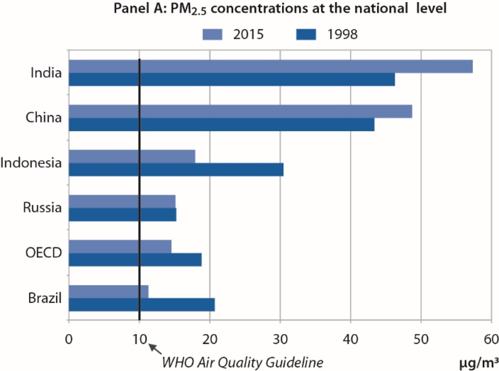
A similar observation can be made for PM pollution, for which NOx and NH3 are precursors. Despite improvements, the populations of most EU countries remain chronically exposed to harmful levels of PM.8 Fewer than one in three OECD countries comply with the WHO Air Quality Guideline for annual average fine particles (PM2.5) exposure of 10 micrograms per m3 (OECD, 2017). Outside the OECD area, exposure to PM2.5 exposure in China and India continued to increase despite already extremely high levels (Figure 3.4). The number of premature deaths from PM2.5 has been increasing between 2000 and 2015, both in emerging countries and OECD countries as a whole (Roy and Braathen, 2017).

Panel A: Average concentrations of fine particles (PM2.5) are derived from satellite observations, chemical transport models and monitoring stations.
Panel B: Annual average concentrations of coarse particles (PM10) for cities with population over 100 000.
Source: OECD (2017 for Panel A; 2012 for Panel B).
The US Environmental Protection Agency’s Science Advisory Board (USEPA-SAB) assessment mapped the risk of nitrogen aerosol deposition in the United States. As evidenced by the assessment, it can be expected than ammonium (NH4+) wet deposition occurs near or downwind of major agricultural centres, and that nitrate (NO3-) levels in wet deposition are consistent with NOx emissions9 (USEPA-SAB, 2011). Increased use of IPA would better correlate nitrogen aerosol risk areas with NOx and NH3 emission zones, thus facilitating policy decision.
Ground-level ozone (GLO)
A similar observation can be made for GLO pollution, for which NOx is a precursor. Despite improvements, the populations of most EU countries remain chronically exposed to harmful levels of GLO (Figure 3.5).10 Reduction of NOx emissions has not (linearly) translated into GLO reduction. Instead, GLO trends over recent decades show complex patterns (Cooper et al., 2014).
As with NO2, changes in GLO concentrations will depend not only on the level of precursor emissions, but also on the location of emissions, atmospheric pathways and climatic conditions.11 In particular, GLO concentrations are often higher downwind of urban areas than in urban areas themselves.12
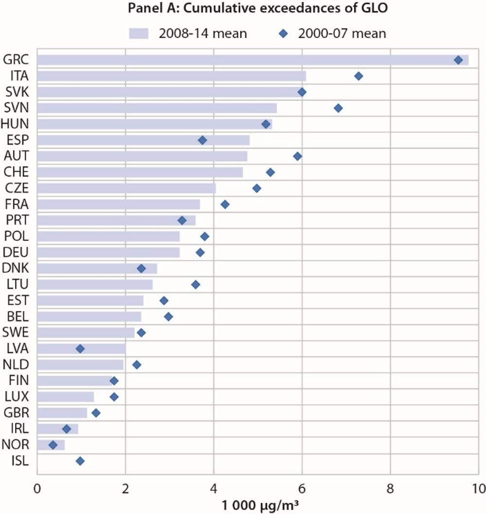

Panel A: Cumulative exceedances of daily maximum 8-hour mean exposures above 70 µg/m3 for all days in a year, based on measurements at ground stations, selected European countries. By comparison, World Health Organisation (WHO) Air Quality Guideline and European Union (EU) target values are, respectively, 100 µg/m3 and 120 µg/m3 for maximum daily 8-hour mean exposure.
Panel B: Annual average GLO concentrations for cities with population over 100 000.
Source: OECD (2017 for Panel A; 2012 for Panel B).
3.2 Case study 2: Impact-Pathway Analysis (IPA) and water pollution
3.2.1 Coastal water pollution
The Chesapeake Bay Watershed covers 90 000 square miles (23 million hectares) across six U.S. States (Delaware, Maryland, Pennsylvania, New York, Virginia, West Virginia) and Washington D.C. Land use is forest (64%), agriculture (24%), urban (8%) and other (4%). Nitrogen, phosphorus and sediment loads delivered from the watershed to the tidal waters of the Bay are the primary concern. They translate into low to no dissolved oxygen (DO) in the Bay and tidal rivers every summer. Required DO levels have been established for the different species living in the Bay as a function of the depth of the water (Figure 3.6).
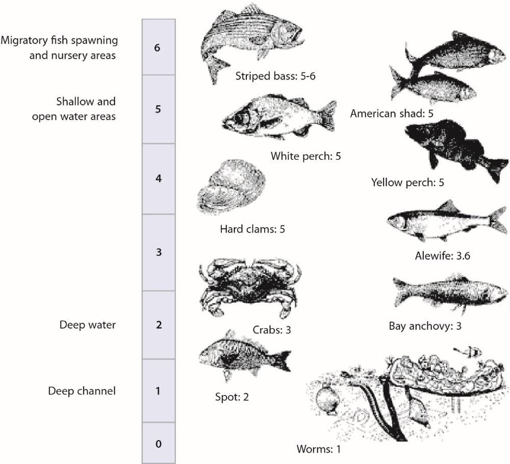
Note: The scale from 1 to 6 is based on the minimum amount of oxygen (mg/l) required for the survival of species.
Source: Linker et al. (2016).
In December 2010, a TMDL of nitrogen and phosphorus allowed to enter the tidal Bay has been set to comply with DO standards. The TMDL covers major land-based sources of nutrients in the watershed (agriculture, sewage) and atmospheric deposition of nitrogen in the watershed. It is the first TMDL scheme in the United States that takes into account atmospheric deposition of nitrogen. The projected reduction in NOx emissions at the national level (pursuant to the Clean Air Act) is deducted from the TMDL, thereby reducing the nutrient reduction effort required from land-based sources. Another TMDL has been established for direct atmospheric deposition of nitrogen in tidal waters.
The relevant “airshed” – the area where emission sources contribute most to deposition in the Bay's watershed – was delineated for each nitrogen form to model nitrogen deposition. The NH3 airshed is similar to the NOx airshed, but slightly smaller (Figure 3.7). Both airsheds are approximately nine times larger than the Bay watershed. Approximately 50% of nitrogen deposits in the Bay come from sources located in the Bay watershed. Another 25% comes from the remaining area in the Bay airshed. The final 25% comes from net ocean exchange.
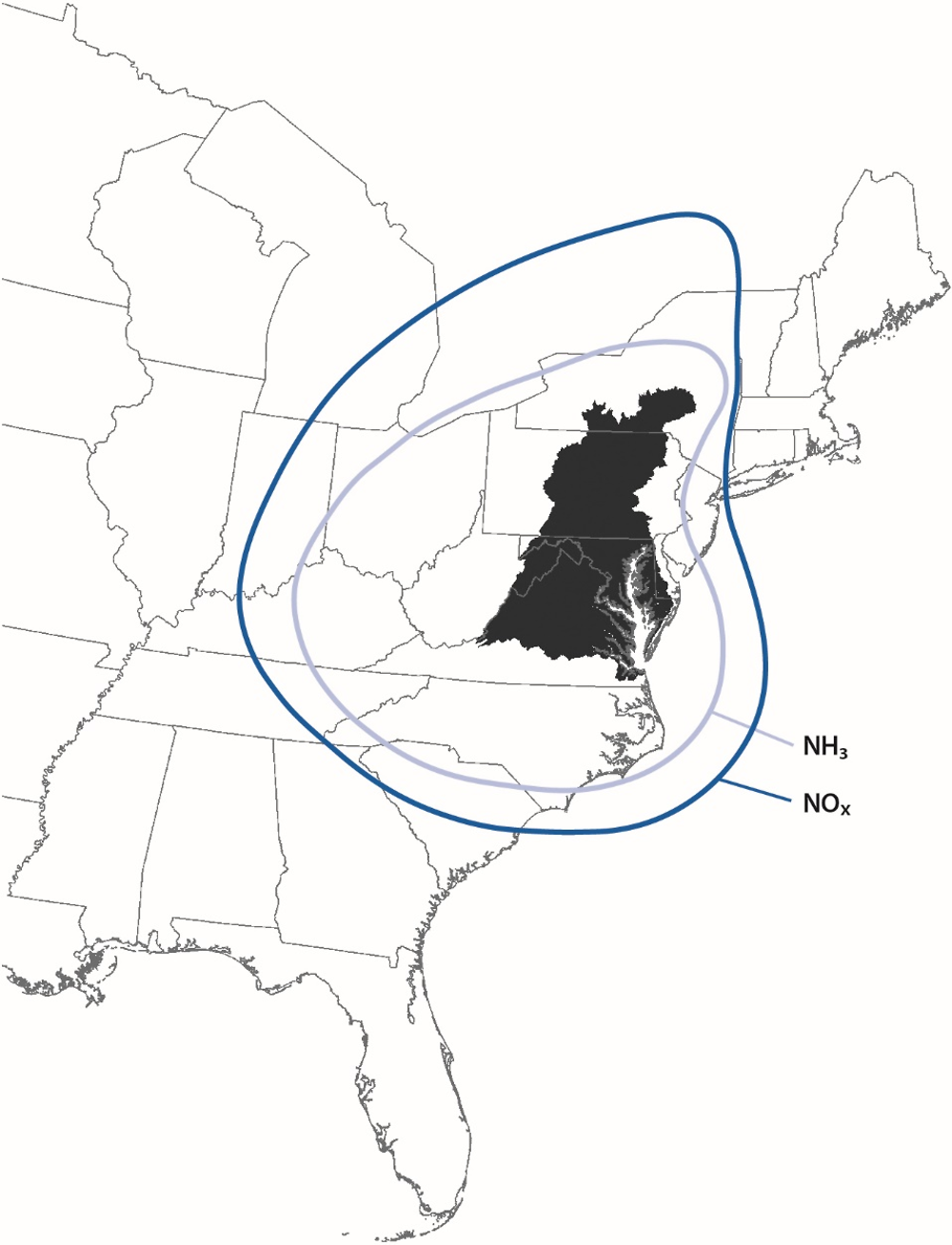
Note: The highlighted area within the airsheds represents the area of the Chesapeake Bay watershed.
Source: Linker et al. (2016).
Integrated modelling supports IPA analysis. It involves a step-by-step approach. First, data from a land use change model, an airshed model and a “scenario builder" software are transmitted to a watershed model (Figure 3.8). The Land Use Change model predicts changes in land use, sewerage, and septic systems given changes in land use policy. The Airshed Model, a national application of Community Multiscale Air Quality Model (CMAQ), predicts changes in deposition of inorganic nitrogen due to changes in emissions.13 The “scenario builder” software combines the output of these models with other data sources, such as the U.S. census of agriculture, to generate inputs to the Watershed Model.

Source: www.chesapeakebay.net/who/group/modeling_team, accessed 11 April 2018.
The Watershed Model then predicts the loads of nitrogen, phosphorus, and sediment that result from the given inputs.14 The estuarine Water Quality and Sediment Transport Model (WQSTM) (also known as the Chesapeake Bay Model) predicts changes in Bay water quality due to the changes in input loads provided by the Watershed Model.15 As a final step, a water quality standard analysis system examines model estimates of DO, chlorophyll, and water clarity to assess in time and space the attainment of the Bay water quality standards
Direct deposition of nitrogen in tidal waters is estimated on the basis of reductions at the federal level of mobile emissions and pursuant to the Cross-State Air Pollution Rule16 plus reductions at the State level.17 NOx deposits on tidal waters have declined since the mid-1980s while NH3 deposits are stable or increasing (Table 3.1). The TMDL target was set at 15.7 million pounds (7 100 tonnes) of N by 2020, representing a 40% reduction in nitrogen deposition compared to 1985.
The combined management of atmospheric and land-based nitrogen inputs in Chesapeake Bay reflects the reality of the nitrogen cycle. Such an IPA makes the risk management of hypoxia in the bay more cost effective. The Chesapeake Bay Programme has been effective as a whole since the TMDL was introduced, although progress remains to be made to meet the nitrogen load target of 2025 (Table 3.2). Estimated nitrogen loads in the Bay watershed decreased by 9% between 2009 and 2016. Agriculture accounts for 42% of the remaining nitrogen loads, followed by discharges from urban runoff and sewage (33%) and atmospheric deposition (25%) (Table 3.2).
More generally, models that predict how nitrogen from the air is deposited in the sea could be useful for managing the risk of algal blooms. For example, researchers have simulated nitrogen deposition in the North Sea and suggested that by superimposing weather forecast data, it would be possible to predict algal blooms (Djambazov and Pericleous, 2015).
3.2.2 Lake water pollution
As nitrogen moves into groundwater to a lake, leaching from different parts of the lake basin reaches the lake at different times and the damage (e.g. eutrophication) is temporally differentiated. Like spatial differentiation in the previous example (Chesapeake Bay), a policy that incorporates time differences is likely to be more cost-effective than a policy that does not. This is what recent studies have sought to demonstrate.
Cox et al., 2013 undertook a simplified analysis of agricultural nitrogen transport pathways through the groundwater system to manage NO3- pollution risk of Lake Rotorua. A geophysical model was used to estimate mean groundwater residence times at the parcel level in the lake basin (Figure 3.9). The authors suggest that time-specific regulation is cost-effective in watersheds where nitrogen transport to the lake is primarily through groundwater (and not runoff) and where transport times are highly differentiated.
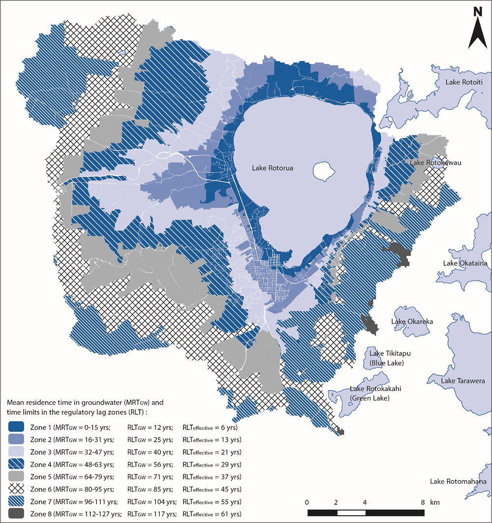
Source: Cox et al. (2013).
"Vintage Nitrogen Trading" (VNT) can be a cost-effective eutrophication risk management tool for lakes for which IPA can predict nitrogen inputs over time (in part, following Anastasiadis et al., 2013). In a vintage trading scheme, the regulator provides a supply of allowances for each vintage year, where the vintage year corresponds to the year when nitrogen will arrive in the lake. Allowances therefore represent rights to contribute to lake loads in a particular year which equate to conditional rights to leach nitrogen from farms18 depending on groundwater lag time. Under regulation, farmers must surrender allowances each year to cover the lake loads that will be caused some time in the future by the nitrogen lost from their property that year.
Under such VNT scheme, each year farmers would need to match their leaching with allowances from the vintage that corresponds to the current year plus their lag time. For example, suppose a farmer with a lag time of 30 years leaches 100 kg of nitrogen in 2018; he would need, in 2018, surrender 100 kg of 2048 vintage allowances. Nitrogen also travels via soil surface runoff (quick-flow). Suppose 50% of nitrogen travels via runoff and 50% via groundwater. Then, the farmer would need, in 2018, surrender 50 kg of 2018 vintage allowances and 50 kg of 2048 vintage allowances.
Any catchment with groundwater lags will have a legacy load: nitrogen in the groundwater from historical leaching that is yet to be realised as lake loads. As it is very difficult to prevent nitrogen already in the groundwater from reaching the lake, regulators must account for legacy loads when setting environmental targets for all sources of nitrogen. This is frequently done by a gradual strengthening of the environmental target over time. Anastasiadis et al., 2011 discuss the design of regulation that allows for legacy loads.
The ability to respond (adaptability) to change is an important feasibility criterion for VNT systems, which require a long period of implementation. Like all tradable permit instruments, VNT systems offer great flexibility in how to reduce nitrogen and where (in the lake basin) to meet the cap. However, once implemented, it may be difficult to revise the cap down (for example, if new evidence on lake water quality emerges). This problem may to some extent be mitigated by the use of "phases" defined in advance, after which modifications of the cap can be introduced to be applied in the following phases (Drummond et al., 2015).
3.2.3 Groundwater contamination
In Oregon, United States, in 2004, the Southern Willamette Valley (SWV) was declared a groundwater management area (GWMA) due to the high concentration of NO3- that has been found in many private wells, with concentrations often exceeding the drinking water standard (10 mg/l). In fact, the SWV-GWMA - 230 square miles (almost 60 000 ha) - has not been delineated on a scientific basis (on the basis of an IPA) but according to criteria of administrative feasibility; it is the area in which public water systems abstract their drinking water.19
The administrative boundaries of the SWV-GWMA do not coincide with the risk area or the emission zone within the meaning of the IPA. It would be more appropriate to delineate the Willamette Lowland area (as a hydrogeological entity) – and not just a portion as is the case with SWV-GWMA – to manage the risk of groundwater contamination in the Willamette Basin (Box 3.1). Indeed, NO3- contamination is only for shallow groundwater - the shallow portion of the Willamette Aquifer adjacent to the Willamette River, known as the “alluvial aquifer”.20
Instead, SWV-GWMA focuses on the protection of public water systems and it is assumed that each public water system has its own pathways of contamination. This led to the delineation of protection zones around each public well (the drinking water protection zones). "Source water assessments" identify potential sources of contamination in the drinking water protection zone (e.g. agriculture, septic tanks, abandoned wells, high density housing) and assign a level of risk (high, medium or low) based on general criteria developed by the USEPA.
This is a kind of IPA but on the wrong scale. Using the terminology of the IPA, the "risk area" is the alluvial aquifer and the "emission zone" is the Willamette Lowland area. Given the connectivity between the alluvial aquifer and the Willamette River, risk management focused on the alluvial aquifer would promote synergy between groundwater quality protection measures and surface water quality protection measures (such as TMDL).
Conlon et al., 2005 estimated the recharge pathways of the Willamette Aquifer using the Precipitation-Runoff Modelling System (PRMS). The PRMS model shows high levels of groundwater recharge in the Coast Range, Western and High Cascade areas. However, it is likely that rainwater will only seep to a shallow depth and then flow into the streams of these areas. From the basin's point of view, this infiltration is not a recharge of the groundwater but a superficial flow in the soil zone. It follows that most of the precipitation in the Coast Range, Western, and High Cascade areas is discharged into streams in these areas and is not available as a source of groundwater in the lowlands (Figure 3.10). Consequently, shallow groundwater recharge in the lowland area occurs locally.

Note: The Willamette Basin includes a lowland area between the Coast Range and the Cascade Range.
Source: Conlon et al. (2005).
3.2.4 Policy relevance of IPA for water pollution risk management
The example of "ocean dead zones" will serve to illustrate the policy relevance of IPA for water pollution risk management. Dead zones are steadily increasing, including in the OECD area, making the identification of the sources of nutrients that cause them a priority (Box 3.2).
As oxygen supply decreases in bottom waters, concentrations may fall below levels necessary to maintain animal life. This low oxygen condition is known as "hypoxia". Hypoxic areas are sometimes referred to as “dead zones”, a term that was first applied to the hypoxic area of the northern Gulf of Mexico, which receives large amounts of nutrients from the Mississippi and Atchafalaya river basins (Rabalais et al., 2010). When fishermen trawl in these zones little to nothing is caught.
Ocean dead zones are closely associated with anthropogenic activities. The worldwide distribution of dead zones is related to major population centres and watersheds that export large quantities of nutrients.
The negative environmental effects of dead zones include loss of habitat, direct mortality, decreased food resources and altered migration for many fish species (bottom-dwelling and pelagic) (Breitburg et al., 2009). Increasing nutrient loads also affect composition of the phytoplankton (Turner et al., 1998). Dead zones also alter ecosystem services such as nutrient cycling (Sturdivant et al., 2012).
Dead zones vary according to seasons. In temperate latitudes, bottom waters can remain hypoxic for hours to months during summer and autumn. The good news is that coastal marine systems can be restored provided sustained efforts are undertaken to reduce nutrient loads. However, once a coastal marine system develops a dead zone, it often becomes an annual event (Baird et al., 2004).
Available data on dead zones provide compelling evidence of a rapid increase in the fertility of many coastal ecosystems since about 50 years ago. Until the late 1960s, there were scattered reports of dead zones in North America and Northern Europe (Diaz et al., 2013). Two decades later, in the early 1990s, dead zones had become prevalent in North America, Northern Europe and Japan (ibid). In the 2000s, dead zones extended their geographic reach to South America, Southern Europe and Australia (ibid).
Some 884 coastal areas around the world have been identified as experiencing the effects of eutrophication; of these, 576 have problems with hypoxia, 234 are at risk of hypoxia and, through nutrient management, 74 can be classified as recovering (Figure 3.11). This figure does not include the likely many unreported hypoxic areas in the tropics because of the lack of local scientific capacity for their detection (Altieri et al., 2017). It has been estimated that more than 10% of coral reefs are at high risk of hypoxia (ibid).
Ocean dead zones are particularly vulnerable to climate change: according to Altieri and Gedan 2015, almost all dead zones are in regions that will experience at least a 2°C temperature increase by the end of the century. Climate change exacerbates hypoxic conditions by increasing sea temperature, ocean acidification, sea level, precipitation, wind and storms.

-
Hypoxic - Areas with scientific evidence that hypoxia was caused, at least in part, by an overabundance of nitrogen and phosphorus. These areas are called “dead zones”.
-
Eutrophic - Areas that exhibit effects of eutrophication, including elevated nitrogen and phosphorus levels, elevated chlorophyll a levels, harmful algal blooms, changes in the benthic community, damage to coral reefs, and fish kills. These areas are at risk of developing hypoxia. Some of the areas may already be experiencing hypoxia, but lack conclusive scientific evidence of the condition.
-
Improved - Areas that once exhibited low dissolved oxygen levels and hypoxia, but are now improving.
-
BRIICS - Brazil, Russia, India, Indonesia, China and South Africa.
Source: Data collected by Robert Diaz, Virginia Institute of Marine Science, as of 22 June 2018.
UNEP, 2012 has correlated the formation of dead zones in the ocean with the growth of agricultural regions, cities and coastal development. According to UNEP, 2012, “the often inefficient use of fertiliser has resulted in releases of nitrogen and phosphorus into waterways and groundwater, which, together with nutrient losses from manure and inadequate sewage treatment has resulted in a substantial increase in nutrient discharges both directly in the coastal water and via rivers receiving emissions from upstream population centres and agriculture".
However, dead zones remain a concern even in the OECD area despite improvements in the efficiency of nitrogen use and improved nitrogen budgets in agriculture in the 2000s (Figure 3.12). As with the Chesapeake Bay mentioned above (see Section 3.2.1), the creation of dead zones is not only due to agriculture or land-based sources. An analysis of the different sources of export of river nitrogen to the sea shows that the sum of atmospheric deposition and natural biological fixation actually exceeds agricultural inputs, with the share of wastewater being the lowest (Table 3.3).21 It is necessary to identify the different sources of nitrogen, their emission zones and the effective tools to manage the risk of dead zones they create, a role for the IPA.
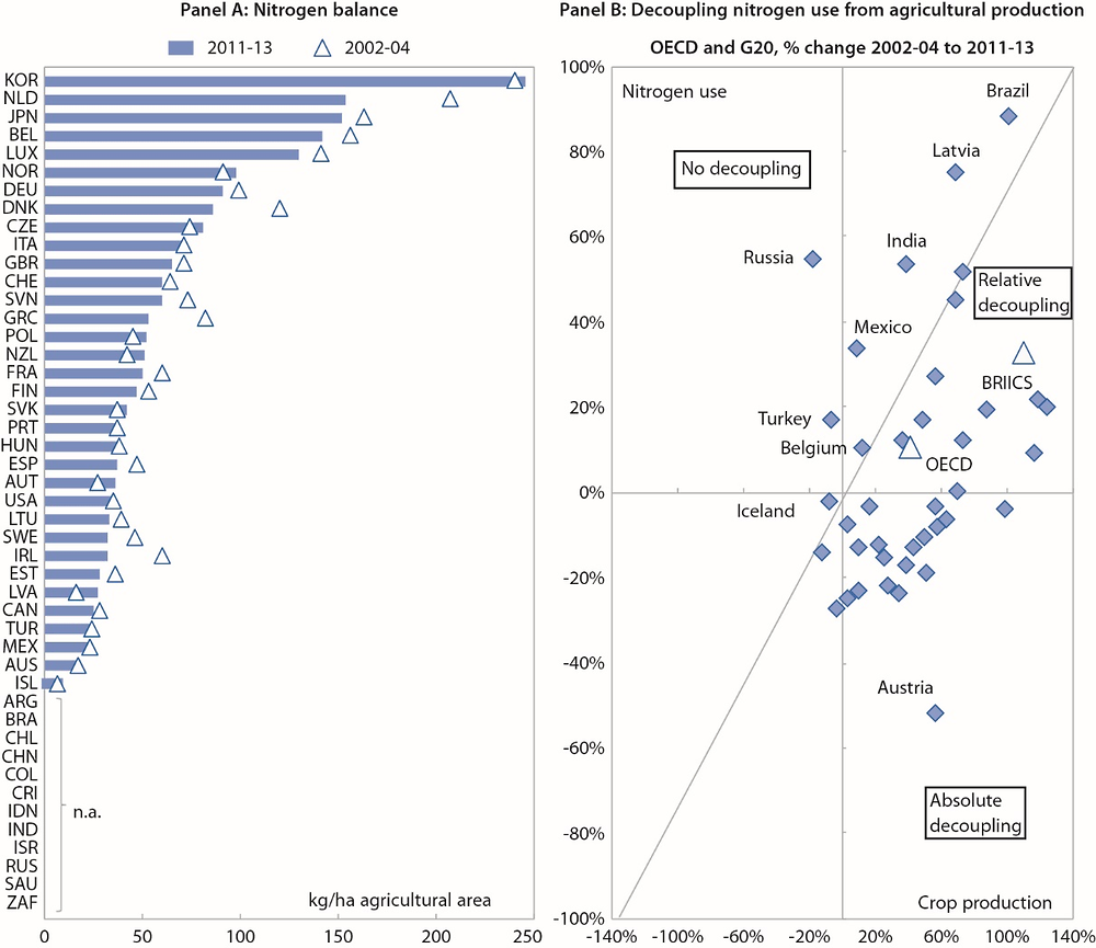
Panel A: National balance at soil surface.
Panel B: Consumption of commercial fertilisers in kg/ha of agricultural area. Crop production value in USD using 2010 prices and PPPs. OECD excludes the Czech Republic.
Source: OECD (2017).
References
Altieri, A.H. et al. (2017), “Tropical Dead Zones and Mass Mortalities on Coral Reefs”, Proc Natl Acad Sci U S A., 114(14).
Altieri, A.H. and K.B. Gedan (2015), “Climate Change and Dead Zones”, Global Change Biology, 21.
Anastasiadis, S. et al. (2011), “Does Complex Hydrology Require Complex Water Quality Policy? NManager Simulations for Lake Rotorua”, Working Paper 11-14, Motu Economic and Public Policy Research, Wellington, doi.org/10.2139/ssrn.1975569.
Anastasiadis, S. et al. (2013), “Does Complex Hydrology Require Complex Water Quality Policy?”, Australian Journal of Agricultural and Resource Economics, 58(1), doi/10.1111/1467-8489.12024/epdf.
Baird, D. et al. (2004), “Consequences of Hypoxia on Estuarine Ecosystem Function: Energy Diversion from Consumers to Microbes”, Ecological Applications, 14(3).
Breitburg, D.L. et al. (2009), « Hypoxia, Nitrogen, and Fisheries: Integrating Effects Across Local and Global Landscapes”, Annual Review of Marine Science, 1.
Conlon, T.D. et al. (2005), Ground-Water Hydrology of the Willamette Basin, Oregon, U.S. Geological Survey, Scientific Investigations Report 2005–5168.
Cooper, O.R. et al. (2014), “Global Distribution and Trends of Tropospheric Ozone: An Observation-based Review”, Elementa: Science of the Anthropocene, 2(29).
Cox, T.J. et al. (2013), “An Integrated Model for Simulating Nitrogen Trading in an Agricultural Catchment with Complex Hydrogeology”, Journal of Environmental Management, 127 (2013), doi.org/10.1016/j.jenvman.2013.05.022.
Diaz, R.J. et al. (2013), “Hypoxia”, in: Noone, K.J. et al. (eds.), Managing Ocean Environments in a Changing Climate, Elsevier, New York.
Díaz, R.J. and R. Rosenberg (2008), “Spreading Dead Zones and Consequences for Marine Ecosystems”, Science, 321.
Djambazov, G. and K. Pericleous (2015), “Modelled Atmospheric Contribution to Nitrogen Eutrophication in the English Channel and the Southern North Sea”, Atmospheric Environment, 102, do.org/10.1016/j.atmosenv.2014.11.071.
Drummond, P. et al. (2015), “Policy Instruments to Manage the Unwanted Release of Nitrogen into Ecosystems – Effectiveness, Cost-Efficiency and Feasibility”, paper presented to the Working Party on Biodiversity, Water and Ecosystems at its meeting on 19-20 February 2015, ENV/EPOC/WPBWE(2015)8.
EEA (2016), Air Quality in Europe — 2016 Report, EEA Report N° 28/2016, European Environment Agency, Copenhagen, doi.org/10.2800/80982
Gauger, Th. (2017), “Reaktiver Stickstoff in der Atmosphäre von Baden-Württemberg - Interimskarten der Ammoniakkonzentration und der Stickstoffdeposition (Depositionsbericht 2017)”, Kapitel 1-4, Landesanstalt für Umwelt Baden-Württemberg, Fachdokumentendienst Umweltbeobachtung, ID U46-S7-J16, Ministerium für Umwelt, Klima und Energiewirtschaft Baden-Württemberg [Ed.], Karlsruhe, Germany, http://www.fachdokumente.lubw.baden-wuerttemberg.de/servlet/is/121207/U46-S7-J16.pdf?command=downloadContent&filename=U46-S7-J16.pdf&FIS=91063.
HELCOM (2013), Summary Report on the Development of Revised Maximum Allowable Inputs (MAI) and Updated Country Allocated Reduction Targets (CART) of the Baltic Sea Action Plan, Helsinki Commission, Helsinki.
Karl, T. et al. (2017), “Urban Eddy Covariance Measurements Reveal Significant Missing NOx Emissions in Central Europe”, Scientific Reports, 7(2536), doi.org/10.1038/s41598-017-02699-9.
Linker, L.C. et al. (2016), “Integrating Air and Water Environmental Management in the Chesapeake Bay Program”, presentation to the Joint OECD/TFRN Workshop on The Nitrogen Cascade and Policy – Towards Integrated Solutions, OECD, Paris, 9-10 May 2016.
LUBW (2018), “StickstoffBW”, Landesanstalt für Umwelt Baden-Württemberg [Ed.], https://www.lubw.baden-wuerttemberg.de/medienuebergreifende-umweltbeobachtung/stickstoffbw.
LUBW (2016), “Beurteilung der Stickstoffdeposition in Baden-Württemberg -- Kurzmitteilung 1/2016 für eine zwischen Bund und Ländern abgestimmte Stickstoffstrategie”, Landesanstalt für Umwelt Baden-Württemberg, Fachdokumentendienst Umweltbeobachtung, ID U10-S7-J16, Ministerium für Umwelt, Klima und Energiewirtschaft Baden-Württemberg and Ministerium für Verkehr und Infrastruktur Baden-Württemberg [Ed.], Karlsruhe, Germany, www.fachdokumente.lubw.baden-wuerttemberg.de/servlet/is/116484/U10-S7-J16.pdf?command=downloadContent&filename=U10-S7-J16.pdf.
Ministry of Economic Affairs (2015), Programma Aanpak Stikstof website, pas.natura2000.nl/ (accessed 27 January 2017).
OECD (2017), Green Growth Indicators 2017, OECD Publishing, Paris, doi.org/10.1787/9789264268586-en.
OECD (2015), Environment at a Glance 2015: OECD Indicators, OECD Publishing, Paris, doi.org/10.1787/9789264235199-en.
OECD (2012), OECD Environmental Outlook to 2050: The Consequences of Inaction, OECD Publishing, Paris, doi.org/10.1787/9789264122246-en.
OECD (2008), OECD Environmental Outlook to 2030, OECD Publishing, Paris, doi.org/10.1787/9789264040519-en.
Pinho, P. et al. (2016), “Mapping Portuguese Natura 2000 Sites in Risk of Biodiversity Change Caused by Nitrogen Pollution”, contribution to the joint OECD/TFRN Nitrogen Workshop, Paris, 9 10 May 2016, Centre for Ecology, Evolution and Environmental Changes and CERENA, Lisbon, Portugal.
PRIMEQUAL (2015), Agriculture et Pollution de l’Air : Impacts, Contributions, Perspectives, État de l’Art des Connaissances), plaquette résumant un séminaire national organisé le 2 juillet 2014 réunissant des experts du Ministère de l’Écologie, du Développement durable et de l’Énergie, de l’Agence de l’Environnement et de la Maîtrise de l’Énergie et de l’Institut national de la recherche agronomique, Programme de Recherche Inter-organisme pour une Meilleure Qualité de l’Air.
Rabalais, N.N. et al. (2010), Dynamics and Distribution of Natural and Human-caused Hypoxia”, Biogeosciences, 7.
Roy, R. and N. Braathen (2017), "The Rising Cost of Ambient Air Pollution thus far in the 21st Century: Results from the BRIICS and the OECD Countries", OECD Environment Working Papers, N° 124, OECD Publishing, Paris, doi.org/10.1787/d1b2b844-en.
Salomon, M. et al. (2016), “Towards an Integrated Nitrogen Strategy for Germany”, Environmental Science & Policy, 55 (2016).
SRU (2015), Nitrogen: Strategies for Resolving an Urgent Environmental Problem, German Advisory Council on the Environment, Berlin.
Sturdivant, S.K. et al. (2012), “Bioturbation in a Declining Oxygen Environment, in situ Observations from Wormcam”, PLoS ONE, 7(4).
Thunis, P. et al. (2017), Urban PM2.5 Atlas - Air Quality in European Cities, European Commission, Joint Research Centre, JRC108595, EUR 28804 EN, Publications Office of the European Union, Luxembourg.
Turner, R.E. et al. (1998), “Fluctuating Silicate: Nitrate Ratios and Coastal Plankton Food Webs”, Proc Natl Acad Sci U S A., 95(22).
UNEP (2012), Green Economy in a Blue World, UNEP, FAO, IMO, UNDP, IUCN, WorldFish Center, GRIDArendal, undp.org/content/dam/undp/library/EnvironmentandEnergy/WaterandOceanGovernance/Green_Economy_Blue_Full.pdf.
USEPA-SAB (2011), Reactive Nitrogen in the United States: An Analysis of Inputs, Flows, Consequences and Management Options, U.S. Environmental Protection Agency’s Science Advisory Board, EPA-SAB-11-013, USEPA, Washington D.C., yosemite.epa.gov/sab/sabproduct.nsf/WebBOARD/INCFullReport/$File/Final%20INC%20Report_8_19_11(without%20signatures).pdf.
Vieno, M. et al. (2016), “The UK Particulate Matter Air Pollution Episode of March-April 2014: More than Saharan Dust”, Environmental Research Letters, 11(4).
Notes
← 1. In 2009, some 48% of Germany’s natural and semi-natural terrestrial ecosystems were affected by eutrophication and 8% were affected by acidification (SRU, 2015).
← 2. For example, many bodies of groundwater still fail to achieve good chemical status according to the EU Water Framework Directive (WFD) due to excessive nitrate (NO3-) concentrations (>50 mg/l). Similarly, many rivers still exceed the WFD good chemical status of 2.5 mg/l NO3- and very few meet the WFD good ecological status due to altered morphology and eutrophication.
← 3. For example, eutrophication remains a problem for almost the entire Baltic Sea (HELCOM, 2013).
← 4. www.aerius.nl/files/media/Publicaties/Documenten/aerius_the_calculation_tool_of_the_dutch_integrated_approach_to_nitrogen.pdf.
← 5. NO2 is directly harmful to human health (see Annex A).
← 6. europa.eu/rapid/press-release_IP-17-238_en.htm.
← 7. Until now NOx emission levels were mainly calculated by collecting emission data at laboratory testing facilities and subsequently extrapolating them in models. However, the amount of pollutant emissions that vehicles emit on a daily basis depends on numerous factors, for example on individual driving behaviour.
← 8. In 2014, respectively 16% and 8% of the EU-28 urban population were exposed to coarse particles (PM10) and fine particles (PM2.5) levels above the EU limit values; the proportions increase to 50% and 85% when considering the more stringent WHO Air Quality Guideline values (EEA, 2016).
← 9. Although the decreases in deposition are probably not linearly proportional to the decreases in emissions. For example, a 50% reduction in NOx emissions is expected to result in an approximate 35% reduction in NO3-concentration and deposition (USEPA-SAB, 2011).
← 10. In 2014, 8% of the EU-28 urban population was exposed to GLO levels above the EU target value and 96% to levels higher than the more stringent WHO Air Quality Guideline value (EEA, 2016).
← 11. GLO concentrations peak in summer. There is a large day-do-day variability reflecting meteorological conditions: GLO is highest under stagnant conditions associated with strong subsidence inversions.
← 12. Near emission sources, NOx reduces GLO by titration, while net GLO formation occurs some distance downwind of NOx sources, depending on temperature and atmospheric dispersion.
← 13. The Airshed Model combines a regression model of wet deposition with CMAQ estimates of dry deposition. CMAQ covers the North American continent on a grid of 36 km x 36 km; a finer grid (12 km x 12 km) is used on the Chesapeake Bay watershed.
← 14. The Watershed Model was first developed in 1982; it is now in its fifth development phase.
← 15. The WQSTM Model also tracks the transport of sediments, including their resuspension, by modelling the waves in the Bay estuary.
← 16. The Cross-State Air Pollution Rule addresses air pollution from upwind states that crosses state lines and affects air quality in downwind states. It replaced the Clean Air Interstate Rule in 2015.
← 17. State Implementation Plans to meet National Ambient Air Quality Standards.
← 18. Assuming that the nitrogen loads in the lake come mainly from farmland.
← 19. In Oregon, private wells are not subject to the laws protecting drinking water. Therefore, their owners are not required to adhere to drinking water standards (and are often unaware of contamination issues as NO3- cannot be tasted, seen or smelled).
← 20. There is ample evidence linking high NO3- values with alluvium adjacent to the Willamette River in the 100-year floodplain.
← 21. The relative importance of agricultural sources is projected to increase by 2030 in a business as usual scenario (Table 3.3).