Chapter 5. Inequality in Job Accessibility via Transit in US Cities
This chapter studies patterns in job accessibility via transit, that is the number of jobs that are accessible with a 30-minute commute from a given census tract, across and within 46 US Core Based Statistical Areas (CBSAs). The Gini Index is used to measure inequality in job accessibility. Census and administrative data are used to construct several indices of racial segregation, concentration, and centralisation. The chapter examines the correlation between the observed inequality in job accessibility via transit and the spatial distribution of CBSAs’ residents and jobs, as measured by these indices, as well as economic outcomes such as economic inequality and unemployment. Finally, the chapter characterises tracts enjoying different levels of job accessibility, both in terms of residents’ characteristics and of geographic location within CBSAs.
Introduction
The spatial mismatch hypothesis posits that minorities’ high unemployment rates and low wages are due to the fact that minorities reside in areas with low employment, or low employment growth (Kain, 1965, 1968; Raphael, 1998). After World War II, improvements in road transportation allowed industries with high land and transportation costs to relocate to the suburbs, areas that provided high land availability and proximity to highways (Glaeser and Kahn, 2001). In the US, white households were able to follow jobs to the suburbs, while African-Americans initially faced strong barriers to suburban residence (Boustan and Margo, 2009).
In a review of the literature on spatial mismatch, Ihlanfeldt and Sjoquist (1998) conclude that job accessibility is correlated to employment outcomes. However, causality is hard to establish, given concerns of reverse causality and selection. Moreover, several mechanisms other than commuting might drive the correlation between job accessibility and employment outcomes, such as lack of information about distant jobs, or (perceived) discrimination by employers (Hellerstein et al., 2008).
Public transit infrastructure, including bus and rail, could help mitigate this mismatch by allowing individuals to reach job opportunities located in different neighbourhoods at a low monetary cost. Blumenberg and Pierce (2014) show that beneficiaries of the Moving to Opportunities (MTO) programme who move to a neighbourhood with better public transit access appear to be better able to maintain employment. While beneficiaries’ endogenous selection into neighbourhoods could be correlated with other factors influencing employment histories, this finding might help explain why MTO vouchers appear to have no impact on adult self-sufficiency, employment, earnings, or welfare receipt (Katz et al., 2001; Kling et al., 2007; Ludwig et al., 2013). This chapter examines the extent to which variation in job accessibility by transit is associated to better local economic outcomes, and if so, for whom.
Using data from 100 US Metropolitan Statistical Areas (MSAs), Tomer et al. (2011) document that job accessibility via transit differs considerably across metro areas, reflecting variable transit coverage levels and service frequencies, and variable levels of employment and population decentralisation. Moreover, fewer low- and middle-skill jobs are accessible via transit for the typical metropolitan commuter. These findings are in line with research showing that the recent urban revival is related to shifts in preferences of high skilled workers for amenities as well as for shorter commutes, which has lead them to move closer to Central Business Districts (CBDs) where high-skill jobs tend to be concentrated (Edlund et al., 2015; Couture and Handbury, 2017). Building on these findings, this chapter examines how patterns in job accessibility via transit within Core Based Statistical Areas (CBSAs) relate to inequality and economic outcomes within CBSAs.1
The main data source employed here defines job accessibility by transit as the number of jobs that are accessible with a 30-minute commute by transit from a given census tract. See Annex Table 5.A.1 for a list of data sources. Building on these data, this chapter constructs a measure of inequality in job accessibility by transit, the Gini index, to document the extent to which job accessibility by transit varies within the 46 US CBSAs in the study sample.
Second, this chapter investigates the role that residential and workplace location, as well as geographic and regulatory constraints to housing supply, play in determining the observed inequality in job accessibility via transit. Intuitively, the number of jobs accessible by transit from a given tract depends on the location of jobs within the CBSA and the transit network. Based on the available employment and commuting opportunities and the resulting equilibrium housing prices, households will select where to live. From a policy perspective, it is important to disentangle which factors are more strongly related to inequality in job accessibility.
Third, this chapter investigates the impact inequality in job accessibility via transit has on economic outcomes, both at the CBSA and at the tract level, and asks the following question. To what extent does inequality in job accessibility via transit translate into economic inequality? Finally, this chapter identifies tracts that appear to enjoy better job access as well as those that might be left behind.
Several aspects of urban shape as well as residential and workplace location may matter to understand the implications of inequality in job accessibility by transit. To investigate the importance of the geographic location of homes and jobs, this chapter constructs indicators of residential and job concentration that measure the extent to which people and jobs are more concentrated in certain tracts than land area would suggest. To investigate the relevance of the spatial mismatch hypothesis in accounting for inequality in job accessibility by transit, this chapter constructs indicators of residential and workplace segregation along racial lines that measure the extent to which white and minority households and jobs held by white and minority workers are evenly distributed across census tracts or appear to be segregated.
The main results include the following. In cities where employment is more concentrated, high workplace segregation along racial lines, rather than residential segregation, is associated with high inequality in job accessibility via transit. In these cities, public transit might fail to serve important centres of employment for minorities. Also in these cities, inequality in job accessibility via transit is associated with inequality in unemployment rates across tracts, suggesting that lack of transit might hinder job opportunities for residents of certain neighbourhood. The tract level analysis corroborates this hypothesis. In cities with high levels of workplace segregation, tracts with better access to jobs saw lower rates of growth in unemployment between 2000 and 2010. Tracts with higher minority rates appear to have access to fewer jobs within a 30-minute transit commute, in line with the spatial mismatch hypothesis. In contrast, income levels appear to be negatively correlated with job accessibility by transit reflecting the fact that wealthier households might sort into less served suburbs that are further away from jobs.
The chapter is structured as follows. After this introduction the next section discusses possible measures of job accessibility by transit, provides preliminary evidence on the relationship between inequality in job accessibility and workplace segregation and economic outcomes. The third section investigates which neighbourhoods within a given CBSA appear to suffer the most from poor public connections to jobs, and establishes both the characteristics of residents of tracts with better and worse access to jobs by transit and the location of these tracts located within cities. Finally, the last section concludes.
Inequality in job accessibility by transit across US cities
Measuring inequality in job accessibility by transit
This chapter investigates the role inequality in job accessibility by transit plays in shaping the spatial distribution of economic development in US CBSAs. The primary sub-CBSA unit of observation in this study is the census tract, a small, relatively permanent statistical subdivision of a county or equivalent entity, with a population size between 1 200 and 8 000 people. The data source for the measure of job accessibility counts the number of job accessible with a 30-minute transit commute between centroids of census blocks, statistical subdivisions fully contained within a census tract.2 Transit modes include bus and rail. Travel times are computed using transit schedules valid for January 29, 2014, a Wednesday, and assuming perfect adherence to the schedule and a walking speed of 5 km/hour. Specifically, transit times between destinations are computed for each minute in the time interval between 7am and 9am, and averaged within this interval to take into account transit service frequency. To obtain the tract-level values, this chapter sums the measure for individual blocks within each tract. Finally, to define inequality in job accessibility by transit, the Gini index for this measure is constructed as explained in Box 5.1.
Gini Coefficient: The Gini coefficient is a measure of inequality of a distribution. It is defined as a ratio with values between 0 and 1, where 0 corresponds to perfect equality and 1 corresponds to perfect inequality. The numerator is the area between the Lorenz curve of the distribution and the uniform distribution line; the denominator is the area under the uniform distribution line. To construct the measure of inequality across tracts used in this chapter, each variable of interest is weighted by the share of the CBSA population that resides in the tract. The resulting formula is as follows:
where xi is the tract-level variable of interest, n is the number of tracts in the CBSA, and is the share of the city population, P, that resides in tract i.
Dissimilarity Index: The Dissimilarity index is a measure of segregation that represents the proportion of the population or jobs that would have to move to create a perfectly homogeneous distribution. It ranges between 0 and 100, where 0 indicates an even distribution of minorities, and 100 indicates perfect segregation. The Dissimilarity index is computed as follows:
where ki is the number of people or jobs in the majority group in tract i and K is the number of majority people or jobs in the whole CBSA.
Delta Index: The Delta index is a measure of concentration. It ranges between 0 and 1, where 0 indicates perfectly even distribution and 1 a concentration of all the population or jobs in one local unit only. It is computed as follows:
where is the share of the city population, P, that resides in tract i and is the share of the city area, A, that is included in tract i.
Modified Wheaton Index: The Modified Wheaton index is a measure of centralisation. It ranges between -1 and 1, where -1 indicates an even distribution of the population or jobs across the city, and 1 indicates perfect centralisation. To construct this index each tract’s distance from the Central Business District (CBD) is computed. Annex Table 5.A.1 discusses data sources for tracts and CBD co-ordinates. Then ordering each tract from the closest to the farthest from the CBD, the index is computed as follows:
.
Figure 5.1 shows that there is ample variation across CBSAs in the average number of jobs per capita that are available within a 30-minute transit commute. Specifically, the distribution of job availability is quite left-skewed, with residents of three-quarters of the CBSAs in the sample having access, on average, to fewer than ten jobs per capita within a 30-minute transit commute. Figure 5.2 shows similar variation in the level of inequality in jobs accessibility via transit at the CBSA level.
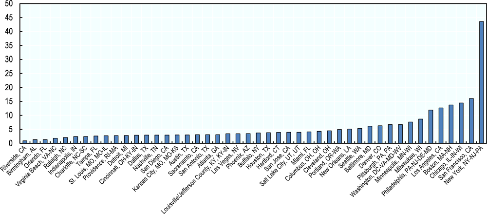
Note: This figure plots the average number of jobs per capita that are available from a CBSA’s census tracts within a 30-minute commute on public transit, with averages calculated weighting by population. CBSAs on the x-axis are ranked based on the available number of jobs per capita within a 30-minute commute on public transit.
Source: Elaborations based on sources detailed in Annex 5.A.
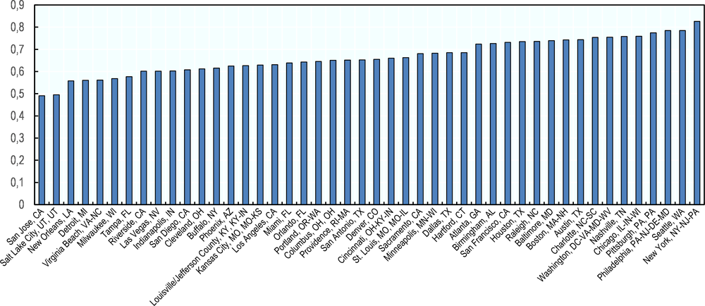
Note: This figure plots the Gini index for average number of jobs per capita that are available from a CBSA’s census tracts within a 30-minute commute on public transit weighted by the tract’s population share. CBSAs on the x-axis are ranked based on the weighted Gini index for the number of jobs per capita within a 30-minute commute on public transit.
Source: Elaborations based on sources detailed in Annex 5.A.
Workplace segregation is associated with inequality in job accessibility by transit
The measure of job accessibility by transit describes the interaction between the location of jobs within a CBSA and the extent of the transit network. Moreover, households select which neighbourhood they want to live in based on the available employment and commuting opportunities (Alonso, 1964; LeRoy and Sonstelie, 1983; Muth 1969). As CBSAs evolve, local governments invest in public transit based on the needs of their constituency. Thus, households’ residence and employment location decisions, as well as public investments in transit infrastructure, are jointly determined in equilibrium. This section explores the characteristics of CBSAs that have a more unequal distribution of job accessibility via transit along these different equilibrium dimensions. Specifically, this section looks at the role played by workplace and residential location choices, as well as housing policies.
The main goal of this analysis is to investigate the extent to which the spatial distribution of jobs and residences might explain inequality in job accessibility by transit. Census data are used to describe the socioeconomic characteristics of tract residents, and matched employer-employee administrative records to derive the spatial distribution of jobs.3 Annex Table 5.A.1 provides more details about these data sources. The main focus of this chapter is segregation along racial lines, both at the workplace and at the residential level, as measured by dissimilarity indices. For the purposes of this work, the population was divided between non-Hispanic whites and minorities. In addition, this section explores the role played by workplace and residential concentration and centralisation, as measured by Delta and Modified Wheaton indices respectively. Box 4.1 details the construction of these indices.
Finally, this section investigates the role played by land availability and land use regulations in determining residential and job locations. For example, areas with less land available for development due to geographic constraints will tend to be more spatially concentrated, thus simplifying commute by transit (Saiz, 2010). Similarly, stricter land use regulations might increase housing prices and make it more difficult for people to find accessible employment (Saks, 2008).
The left panel of Figure 5.3 shows that a higher index of job dissimilarity along race lines is associated with higher inequality in job accessibility via transit. In other words, cities that have more segregated employment locations exhibit also higher levels of inequality in job accessibility by transit. The right panel of Figure 5.3 shows that, if anything, the opposite appears to be true when segregation is measured according to earnings.
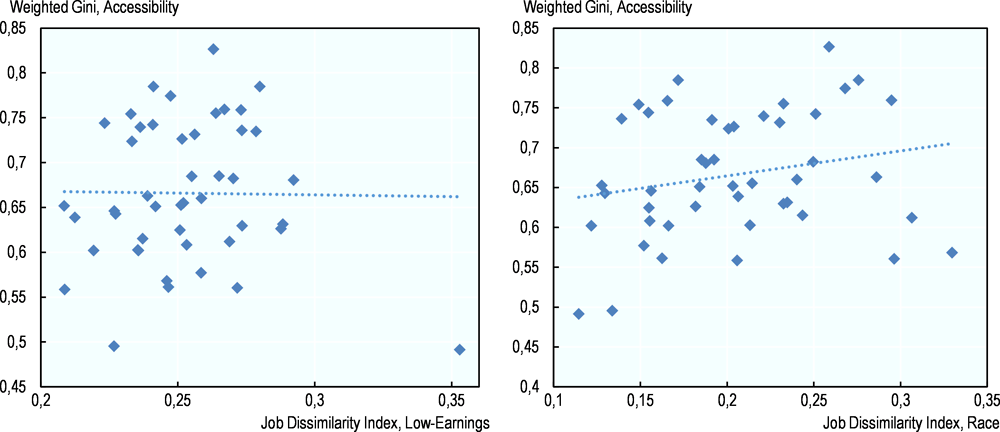
Note: This figure plots CBSA-level Dissimilarity Indices calculated on the characteristics of jobs in each tract on the x-axis against the CBSA-level Gini Index in Job Accessibility by Transit on the y-axis, and fits a linear regression line. Specifically, the left panel constructs a racial Dissimilarity Index, while the right constructs an earnings Dissimilarity Index.
Source: Elaborations based on sources detailed in Annex 5.A.
A potential explanation for the more prominent role of race in explaining inequality in job accessibility via transit is that workplace segregation and residential segregation along racial lines are positively correlated. Indeed, Figure 5.5 presents a similar pattern of positive correlation between residential segregation along racial lines and inequality in job accessibility via transit. Wilson (2008) notes that minority neighbourhoods “typically lack basic services and amenities, such as banks, grocery stores and other retail establishments, parks, and quality transit.” In addition, Raphael and Stoll (2010) remark that among the poor, blacks appear to have suffered more from job suburbanisation. For example poor blacks are less suburbanised than poor whites and Latinos in metro areas with high job sprawl. And those poor black and Latinos who live in the suburbs live disproportionally in jobs-poor communities, particularly in higher-poverty metropolitan areas.
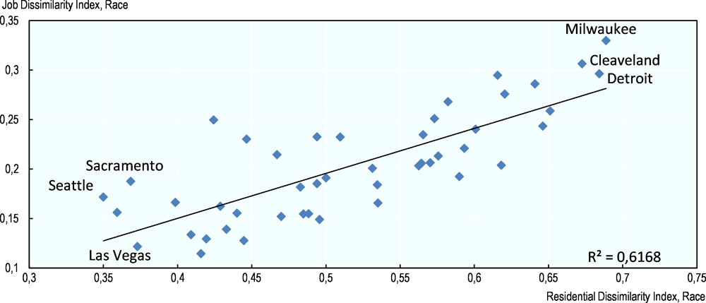
Note: This figure plots CBSA-level racial Dissimilarity Index calculated on the characteristics of residents in each tract on the x-axis against the CBSA-level racial Dissimilarity Index calculated on the characteristics of jobs on the y-axis, and fits a linear regression line.
Source: Elaborations based on sources detailed in Annex 5.A.
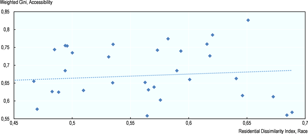
Note: This figure plots CBSA-level racial Dissimilarity Index calculated on the characteristics of residents in each tract on the x-axis against the Gini Index in Job Accessibility by Transit on the y-axis, and fits a linear regression line.
Source: Elaborations based on sources detailed in Annex 5.A.
Workplace segregation along racial lines appears to be strongly positively correlated with inequality in job accessibility by transit also in a regression analysis that considers all predictors of inequality in job accessibility via transit jointly. Figure 5.6 displays the coefficient on workplace segregation in this regression. To investigate the extent to which a city’s productive structure might affect the relationship between workplace segregation and inequality in job accessibility via transit, the regression analysis divides CBSAs according to their degree of job concentration as measured by the Delta Index for jobs. On the one hand, a more dispersed spatial distribution of jobs might allow residents of different neighbourhoods to have easy access to jobs at different locations, resulting in a more equal job access distribution. On the other hand, job agglomeration might allow for better transit planning in a hub and spoke transit system, which is the structure of the transit network in many US CBSAs.
Notably, a comparison of the coefficients displayed in Figure 5.6 shows that the correlation between workplace segregation and inequality in job access is entirely driven by cities with a high concentration of jobs. This finding suggests that high-density employment centres might still lack essential transit connections that would allow minority neighbourhoods to access these jobs.
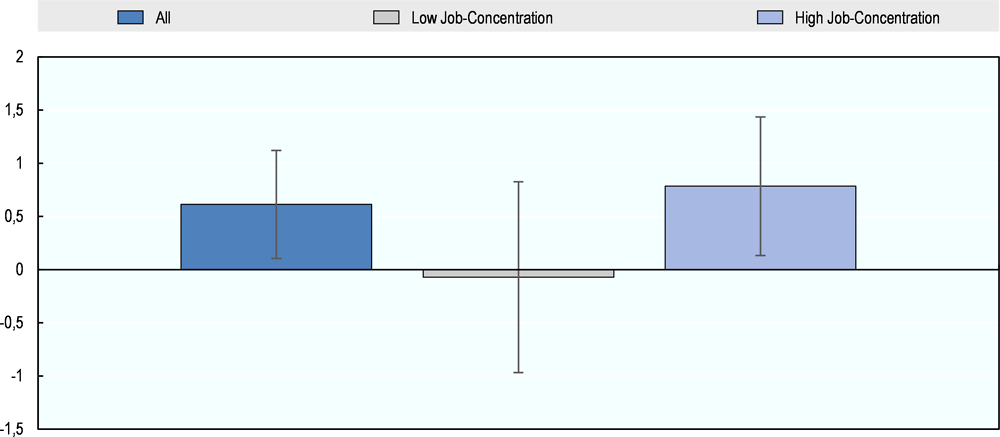
Note: This figure plots the coefficients on the job Dissimilarity Index along racial lines from a CBSA-level regression that includes also the residential Dissimilarity Index along racial lines, the residential Delta Index, the residential Modified Wheaton Index, the job Dissimilarity Index along earnings lines, the job Delta Index, and the job Modified Wheaton Index, as well as controls for population density, the share of land unavailable for development, and a housing Regulatory Index. The dependent variable is the Gini index for average number of jobs per capita that are available from a CBSA’s census tracts within a 30-minute commute on public transit weighted by the tract’s population share. The first bar is estimated on the entire sample of CBSAs, while the second bar is estimated on the sample of CBSAs with a below-median Delta Index for jobs, and the third bar is estimated on the sample of CBSAs with an above-median Delta Index for jobs. The bars represent confidence intervals at the 10% level.
Source: Elaborations based on sources detailed in Annex 5.A.
Table 5.1 presents coefficients for variables describing residential sorting (the first three variables) and job location (rows 4-7).4 Strikingly, when controlling for other CBSA-level factors, residential segregation appears to be negatively correlated with inequality in job accessibility by transit. One potential explanation that is explored further in the within-CBSA analysis below is that residential segregation is correlated with minorities being concentrated in inner cities, which might have better public transit. The fact that workplace segregation appears to be positively correlated with inequality in job accessibility by transit suggests that although minorities might be living in neighbourhoods that are relatively well served after controlling for other socio-demographic characteristics, the jobs available to them might be in areas that have disproportionately worse public transit, lending support to the spatial mismatch hypothesis. Finally, it is worth to reiterate that these results do not appear to be driven by demand for skills. In fact, workplace segregation by earnings does not appear to be significantly correlated with inequality in job accessibility by transit.
This analysis considers also other metrics that describe the spatial distribution of households and jobs within a CBSA, that is, measures of concentration and centralisation of both residential and job locations. Specifically, centralisation indicates high density of people or jobs around the Central Business District (CBD), as identified by the geocode returned when entering the central city name in Google Earth.5 Intuitively, higher residential concentration, as measured by the Delta Index is also associated with lower levels of transit inequality, as conditional on the existing transit network, more people might live close to transportation hubs in a highly concentrated city. Perhaps less intuitively, a high level of job centralisation, as measured by the Modified Wheaton Index is correlated with high levels of inequality in job accessibility by transit. This result suggests that, other things equal, the concentration of employment opportunities near the CBD does not guarantee equality of accessibility. One potential explanation is that urban shape might still play an important role, for example some cities might have multiple centres of employment.
Moreover, as inner cities gentrify and poor and minority residents suburbanise, concentration of jobs near the CBD might not improve job accessibility for some low-income and minority people, as discussed in Raphael and Stoll (2010) and Couture and Handbury (2017). In fact, Schuetz et al. (2017) emphasise that in most metropolitan areas, both central city and suburban neighbourhoods have increasingly become economically and ethnically diverse. Section 4.3 below analyses the characteristics of tracts that are farther from employment opportunities in the CBSA to validate these speculations.
Finally, it is worth noting that housing supply constraints reduce inequality in job accessibility by transit. Intuitively, differences in transit access across tracts are smaller in compact cities. On the other hand, housing regulations do not appear to have any additional explanatory power for inequality in jobs accessibility by transit. This is consistent with the findings that job location matters relatively more for job accessibility than residential sorting.
Inequality in Job Accessibility by Transit and Economic Outcomes
Given the correlation found in the previous section between inequality in job accessibility via transit and workplace segregation, it is natural to ask whether this inequality is reflected in economic outcomes as well. The left panel of Figure 4.7 shows that higher inequality in job accessibility via transit is associated with higher inequality in unemployment rates. The right panel of Figure 5.7 shows that inequality in job accessibility does not necessarily lead to higher levels of unemployment overall at the CBSA level. If anything CBSAs with higher levels of inequality in job accessibility via transit exhibit lower unemployment rates.
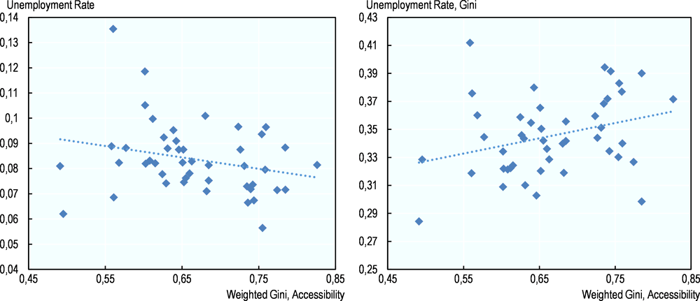
Note: This figure plots the CBSA-level Gini Index in Job Accessibility by Transit on the x-axis against the CBSA-level Gini Index in unemployment rate (left panel) and the CBSA-level average unemployment rate (right panel) on the y-axis, and fits a linear regression line.
Source: Elaborations based on sources detailed in Annex 5.A.
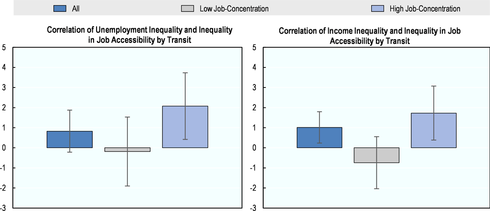
Note: This figure plots the coefficients on unemployment inequality (left panel) and income inequality (right panel) from a CBSA-level regression that includes also average household income, unemployment rate, minority share and Gini Index in minority share, share of high-school dropouts and Gini Index in share of high-school dropouts, share of households with cars and Gini Index in share of households with cars, and population density. The dependent variable is the Gini index for average number of jobs per capita that are available from a CBSA’s census tracts within a 30-minute commute on public transit weighted by the tract’s population share. The first bar is estimated on the entire sample of CBSAs, while the second bar is estimated on the sample of CBSAs with a below-median Delta Index for jobs, and the third bar is estimated on the sample of CBSAs with an above-median Delta Index for jobs. The bars represent confidence intervals at the 10% level.
Source: Elaborations based on sources detailed in Annex 5.A.
A regression analysis confirms that inequality in job accessibility appears to still be correlated with inequality in some economic outcomes after controlling for overall levels. The left panel of Figure 5.8 shows that in CBSAs with above-median levels of job concentration, higher inequality in job accessibility via transit is associated with higher inequality in unemployment rate. One potential explanation for this finding is that in cities where employment is less dispersed, workplace segregation might result in fewer employment opportunities available by transit for residents of minority neighbourhoods, thus creating pockets of unemployment at the neighbourhood level, and giving raise to the observed inequality in unemployment rates at the CBSA level. This channel is analysed further in Section 5.3 below, exploiting data at the census tract level.
In addition, inequality in job accessibility appears to be associated with disparities in income across tracts, as measured by the tract-level Gini Index, as shown in the right panel of Figure 4.8. In contrast, inequality in job accessibility does not appear to be correlated with levels of economic development overall (Table 5.2). Finally, one would expect car ownership rates to respond to the (lack of) availability of transit, creating a positive correlation between inequality in job accessibility by transit and car ownership. In contrast, Table 5.2 shows a negative correlation between levels of car ownership and inequality in job accessibility via transit, suggesting that households might not be able to substitute for the absence of public infrastructure by privately investing in cars.
Inequality in job accessibility via transit within US cities
Access to jobs via public transit is correlated with employment growth
This section investigates which neighbourhoods within a given CBSA appear to suffer the most from poor public connections to jobs. Specifically, this section explores the characteristics of census tracts with different levels of job accessibility by transit within the same CBSA. The sample includes 33 624 census tracts in the 46 CBSAs studied above. Section 4.2.2 above suggests that workplace segregation along racial lines is associated with inequality in job accessibility by transit at the CBSA level. Therefore, the regression analysis distinguishes between cities with below- and above-median levels of workplace segregation as measured by the race Dissimilarity Index.
Tracts that have access to more jobs via public transit have generally been associated with lower rates of growth in unemployment in the years 2000s. In other words, where job opportunities are more segregated, access to public transit appears to enable workers to find and keep employment at higher rates. This pattern is shown in the left panel of Figure 4.9, while the right panel of Figure 4.9 shows that these tracts do not necessarily have lower levels of unemployment in absolute terms. Table 5.3 confirms that this pattern holds also after controlling for tracts’ socioeconomic characteristics and absorbing CBSA fixed effects. Specifically, this relationship holds only in cities with high levels of workplace segregation.
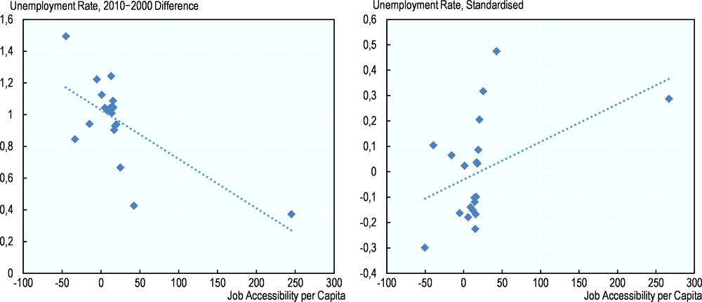
Note: This figure plots the tract-level number of jobs accessible per tract on the x-axis against the tract-level growth in unemployment rate between 2000 and 2010 (left panel) and the tract-level unemployment rate, standardised (right panel) on the y-axis after partialling out CBSA fixed effects, and fits a linear regression line.
Source: Elaborations based on sources detailed in Annex 5.A.
Tracts with better job access have fewer minority residents and are closer to employment centres
This last section asks the following questions. What are the characteristics of residents of tracts with better and worse access to jobs by transit? And where are these tracts located within cities’ geographies?
Tracts with higher minority rates appear to have access to fewer jobs by transit, consistent with the spatial mismatch hypothesis (Figure 5.10). Table 5.3 confirms that this racial pattern holds after controlling for income. In fact, income appears to be negatively correlated with job accessibility by transit, likely reflecting the fact that wealthier households might sort into less served suburbs. To this point, car ownership rates are also negatively correlated with job access via public transit.
Intuitively, geographic location relative to employment centres matters for access to jobs. To analyse the spatial distribution of tracts with better and worse access to jobs within CBSAs, each tract’s distance to the CBD and to the closest economic subcentre is computed. Specifically, tracts with an abnormal job density are identified as economic subcentres, following Veneri (2015). Table 5.4 shows that on average, close to 10% of tracts in a given city are identified as subcentres. Table 5.3 shows that a tract’s distance from the CBD and other employment subcentres is negatively correlated with job access by transit. What’s more, distance to the nearest subcentre appears to matter relatively more than distance to the CBD, suggesting that polycentric cities might result in a more equal distribution of job accessibility.
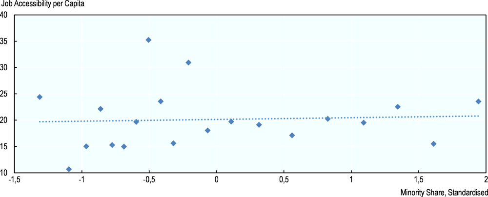
Note: This figure plots the tract-level minority share, standardised, on the x-axis against the tract-level number of jobs accessible per tract on the y-axis after partialling out CBSA fixed effects, and fits a linear regression line.
Source: Elaborations based on sources detailed in Annex 5.A.
The identification of economic subcentres within a CBSA allows to further investigate the spatial mismatch hypothesis and the finding that tracts with higher minority rates appear to have access to fewer jobs by transit. Figure 5.11 shows that the relationship between a tract’s distance from the closes economic subcentre and the share of minorities in that tract is nonlinear. Specifically, for tracts that are relatively close to economic subcentres, the minority share increases with distance.
However, for tracts that are further from economic subcentres than the CBSA’s average, minority share decreases with distance. This pattern confirms that minorities might indeed suffer from poorer connections to jobs than their white counterparts, with the exception of those wealthier households who sort into less served suburbs and commute by car.
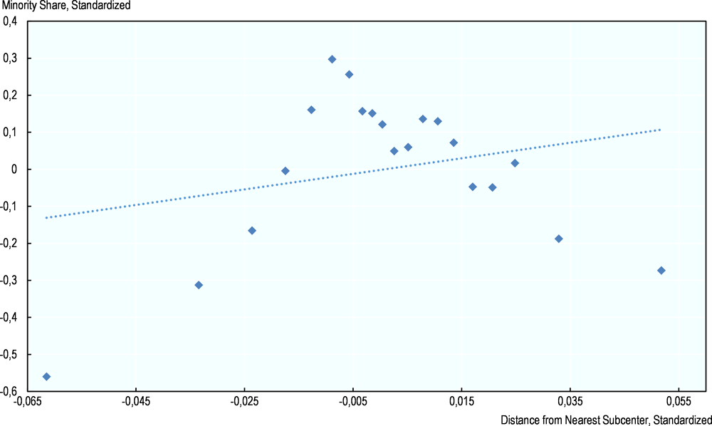
Note: This figure plots tracts’ standardised distance from economic subcentres on the x-axis against the tracts’ standardised minority share on the y-axis, after partialling out CBSA fixed effects, and fits a linear regression line.
Source: Elaborations based on sources detailed in Annex 5.A.
Finally, this section analyses the implications of polycentric CBSAs. As shown above, a high level of job centralisation, as measured by the Modified Wheaton Index is correlated with high levels of inequality in job accessibility by transit. One potential explanation is that when cities have multiple centres of employment, the distance from the CBD might not be the relevant metric for some workers. In fact, job centralisation is only moderately negatively correlated with distance from the nearest subcentre of employment, as shown in Figure 5.12.
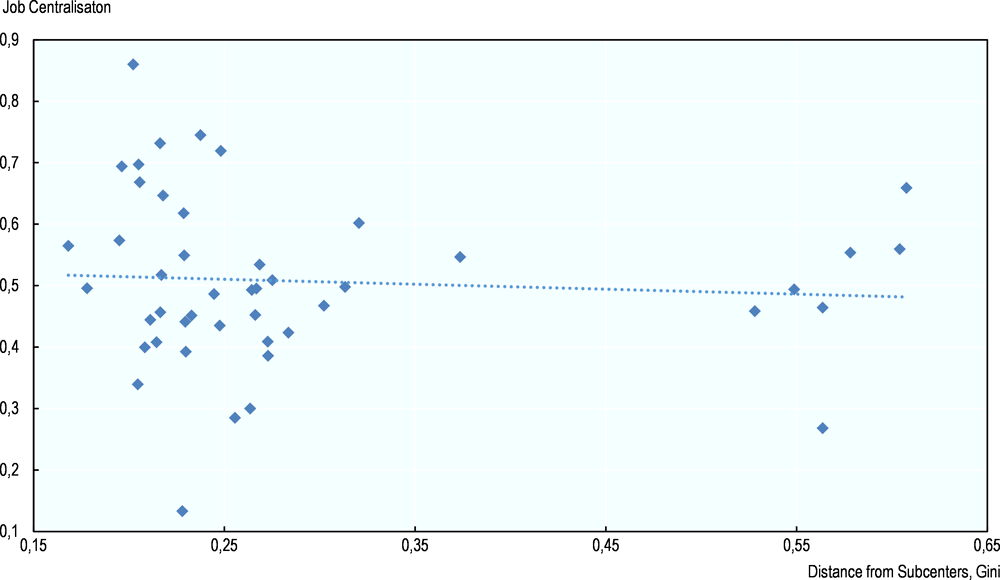
Note: This figure plots CBSA-level Gini Index for tracts’ distance from economic subcentres on the x-axis against the CBSA-level Modified Wheaton Index for jobs on the y-axis, and fits a linear regression line.
Source: Elaborations based on sources detailed in Annex 5.A.
Conclusion
This chapter examines how patterns in job accessibility via transit within 46 US Core Based Statistical Areas (CBSAs) relate to inequality and economic development within CBSAs. This work exploits a variety of administrative and survey data sources for 33 624 census tracts in these 46 CBSAs, including demographic characteristics and employment counts, as well as information on the number of jobs that are accessible with a 30-minute commute by transit from a given census tract. The analysis relies on measures of socioeconomic inequality, as well as a measure of inequality in job accessibility by transit.
First, this chapter documents the extent to which job accessibility by transit varies within the 46 US CBSAs in the sample. Second, it explores the role that residential and workplace location, as well as housing policies, play in determining the observed inequality in job accessibility via transit. Third, this chapter investigates the impact inequality in job accessibility via transit has on economic outcomes, both at the CBSA and at the tract level. Specifically, it studies the extent to which inequality in job accessibility via transit translates into economic inequality. Finally, this chapter asks which tracts appear to enjoy better job access and who, instead, might be left behind.
The results in this chapter show that in CBSAs where there is high inequality in job accessibility by transit, most jobs within a given tract are more likely to be held either by whites or by minorities than the overall CBSA-level racial composition would suggest. In fact workplace segregation along racial lines, rather than residential segregation, exhibits a stronger association with inequality in job accessibility by transit. In these cities, public transit might fail to serve important centres of employment for minorities, thus leading to higher inequality in unemployment rates across tracts. Moreover, in cities with high levels of workplace segregation, tracts with better access to jobs saw lower rates of growth in unemployment between 2000 and 2010. These findings together suggest that lack of transit might hinder job opportunities for residents of certain neighbourhoods. Finally, tracts with higher minority rates appear to have access to fewer jobs by transit, in line with the spatial mismatch hypothesis. In contrast, income levels appear to be negatively correlated with job accessibility by transit reflecting the fact that wealthier households might sort into less served suburbs.
Bibliography
Alonso, W. (1964), Location and Land Use. Toward a General Theory of Land Rent, Harvard University, Cambridge, MA.
Blumenberg, E. and G. Pierce (2014), “A driving factor in mobility? Transportation’s role in connecting subsidized housing and employment outcomes in the moving to opportunity (MTO) program”, Journal of the American Planning Association, 80(1), pp. 52–66.
Boustan, L.P. and R.A. Margo (2009), “Race, segregation, and postal employment: New evidence on spatial mismatch”, Journal of Urban Economics, 65(1), pp. 1–10.
Census Bureau (2018), U.S. Gazetteer Files, https://www.census.gov/geo/maps-data/data/gazetteer.html
Census Bureau (2018), Workplace Area Characteristics Files, LODES Data,
https://lehd.ces.census.gov/data/
Couture, V. and J. Handbury (2017), Urban Revival in America, 2000 to 2010, Mimeo.
Edlund, L., C. Machado and M.M. Sviatschi (2015), Bright Minds, Big Rent: Gentrification and the Rising Returns to Skill, Technical report, National Bureau of Economic Research.
Geolytics (2018) Neighborhood Change Database,
http://www.geolytics.com/USCensus,Neighborhood-
Change-Database-1970-2000,Products.asp
Glaeser, E.L. and M.E. Kahn (2001), “Decentralized employment and the transformation of the American city”, Brookings-Wharton Papers on Urban Affairs, 1, pp. 1–63.
Hellerstein, J. K., D. Neumark and M. McInerney (2008), “Spatial mismatch or racial mismatch?”, Journal of Urban Economics, 64(2), pp. 464–479.
Holian, M. and M. Kahn (2015), Central Business District Geocodes,
http://mattholian.blogspot.com/2013/05/central-business-district-geocodes.html
Ihlanfeldt, K.R. and D.L. Sjoquist (1998), “The spatial mismatch hypothesis: A review of recent studies and their implications for welfare reform”, Housing Policy Debate, 9(4), pp. 849–892.
Kain, J.F. (1968), “Housing segregation, negro employment, and metropolitan decentralization”, The Quarterly Journal of Economics, 82(2), pp. 175–197.
Kain, J.F. (1965), “The effect of the ghetto on the distribution and level of non-white employment in urban areas”, in Proceedings of the Social Statistics Section of The American Statistical Association, Philadelphia, PA.
Katz, L.F., J.R. Kling and J.B. Liebman (2001), “Moving to opportunity in Boston: Early results of a randomized mobility experiment”, The Quarterly Journal of Economics, 116(2), pp. 607–654.
Kling, J.R., J.B. Liebman and L.F. Katz (2007), “Experimental analysis of neighbourhood effects”, Econometrica, 75(1), pp. 83–119.
LeRoy, S. F. and J. Sonstelie (1983), “Paradise lost and regained: Transportation innovation, income, and residential location”, Journal of Urban Economics, 13(1), pp. 67–89.
Ludwig, J., Duncan, G. J., Gennetian, L. A., Katz, L. F., Kessler, R. C., Kling, J. R., & Sanbonmatsu, L. (2013), “Long-term neighbourhood effects on low-income families: Evidence from moving to opportunity”, The American Economic Review, 103(3), pp. 226–231.
McKenzie, B. and M. Rapino (2011), Commuting in the United States: 2009, US Department of Commerce, Economics and Statistics Administration, US Census Bureau, Washington, DC.
Muth, R. (1969), Cities and Housing: The Spatial Patterns of Urban Residential Land Use, University of Chicago Press, Chicago.
Owen, A. and D.M. Levinson (2014), Access across America: Transit 2014, Center for Transportation Studies, University of Minnesota, http://hdl.handle.net/11299/168102.
Raphael, S. (1998), “The spatial mismatch hypothesis and black youth joblessness: Evidence from the San Francisco bay area”, Journal of Urban Economics, 43(1), pp. 79–111.
Raphael, S. and M.A. Stoll (2010), Job Sprawl and the Suburbanization of Poverty, Metropolitan Policy Program at Brookings, Washington, DC.
Saiz, A. (2010), “The geographic determinants of housing supply”, The Quarterly Journal of Economics, 125(3), pp. 1253–1296.
Saks, R. E. (2008), “Job creation and housing construction: Constraints on metropolitan area employment growth”, Journal of Urban Economics, 64(1), pp. 178–195.
Schuetz, J. et al. (2017), Are Central Cities Poor and Non-White?, FEDS Notes, Federal Reserve System, Washington, DC, https://doi.org/10.17016/2380-7172.1982.
Tomer, A., Kneebone, E., Puentes, R., and A. Berube (2011), Missed opportunity: Transit and Jobs in Metropolitan America, Brookings Institution, Washington, DC.
Veneri, P. (2015), “Urban Spatial Structure in OECD Cities: is Urban Population Decentralising or Clustering?”, OECD Regional Development Working Papers, No. 2015/01, OECD Publishing, Paris, https://doi.org/10.1787/5js3d834r3q7-en.
Wilson, W.J. (2008), “The political and economic forces shaping concentrated poverty”, Political Science Quarterly, 123(4), pp. 555–571.
Notes
← 1. According to the US Census Bureau, Core Based Statistical Areas (CBSAs) consist of the county or counties or equivalent entities associated with at least one core (urbanised area or urban cluster) of at least 10 000 population, plus adjacent counties having a high degree of social and economic integration with the core as measured through commuting ties with the counties associated with the core. The general concept of a CBSA is that of a core area containing a substantial population nucleus, together with adjacent communities having a high degree of economic and social integration with that core. CBSAs include metropolitan statistical areas and micropolitan statistical areas.
← 2. Owen and Levinson (2014) count the number of jobs within 10, 20, 30, 40, 50, and 60 minutes. However, they only publish data about the number of jobs available within a 30-minute commute, which limits the scope of the analysis in this chapter. According to their study, between a fifth and a tenth of the jobs available within an hour commute are available within a 30-minute commute. For reference, the 2009 American Community Survey data show that workers took an average of 25.1 minutes to get to work, an increase from 1980 when average commute was just under 22 minutes. While 62.2% of workers reported commuting for 29 minutes or less, average commutes by public transit is longer, 47.8 minutes (McKenzie and Rapino, 2011).
← 3. In these data, a place of work is defined by the physical or mailing address reported by employers in the QCEW (formerly ES-202) or Multiple Worksite Reports. In other words, if employers report multiple worksites, jobs are allocated accordingly. However, if employers fail to report these, then all jobs will be allocated to headquarters.
← 4. The regression analysis also controls for population density to account for the fact that less dense cities might rely on different transit networks and might exhibit different residential and job distribution patterns.
← 5. Data on the location of the CBD comes from Holian and Kahn (2015).