Chapter 2. Employment growth of establishments in the Brazilian economy: Results by age and size groups
The general objective of this chapter is to analyse the statistical patterns of employment dynamics of establishments in the Brazilian economy. In particular, with the help of large scale longitudinal plant-level data, we study the life cycle evolution of establishments so that we can assess how their age, as well as their entry and exit components, are related to the employment growth process in the country. Considering a representative establishment, the results show that it is born small (perhaps too small) and that the pattern of the growth rate over its life cycle imposes a long time span to surpass the threshold of a mid-sized plant. Further results confirm that the middle part of the size distribution is “missing” in Brazil and apparently this feature is more intense than in other countries for which there are available and comparable results.
Introduction
Maintaining high employment growth rates over long time periods is considered to be desirable for the development process not only because of its direct effect on aggregate employment growth but also because of the connections with other performance indicators such as wage and productivity growth. The pattern of employment growth is thus a key process to be monitored in any economy, in particular economies of developing countries like Brazil.
Typically, the monitoring of employment growth in a country is implemented using household surveys. Though rich in information on workers’ characteristics, this type of survey rarely contains information on the characteristics of the establishments where they work, such as their size and age. The process of employment growth is, however, closely connected to the characteristics and performance of establishments over their life cycle. For instance, the entry and exit processes of establishments, as well as their capacity to grow, are important components behind the employment dynamic in an economy. Using establishment-level data is thus a highly valuable source of information for a better understanding of aggregate employment growth.
One of the main theoretical arguments for why aggregate employment and other performance indicators are linked to establishments connects their life cycles to a learning process through which the establishment (decision maker) gradually adjusts to the (new) environment right from the beginning of its operations (Nelson and Winter, 1982). This may be motivated by a learning process not only about the evolving environment but also about its own capabilities (Jovanovich, 1982). According to this view, an important indicator to be monitored is the incidence of establishments closing down according to establishment age, which represents an interruption of the learning process.
Given this background, the general objective of this chapter is to analyse the statistical patterns of employment dynamics of establishments in the Brazilian economy. In particular, with the help of large scale longitudinal plant-level data this chapters studies the life cycle evolution of establishments so it is possible to assess how their age, as well as their entry and exit components, are related to the employment growth process in the country.
This chapter’s focus will be on the performance of small establishments at birth. Studying the pattern of growth of this segment is important for at least two reasons. First, because any small improvement in the rate of employment growth of small establishments tends to have a considerable impact on job creation due to their large share in the establishment and employment size distributions of countries, in particular developing countries. Second, it has potential effects on the degree of competition in various industries, which in turn affects price adjustments and the innovation impetus in the economy.
The present chapter bridges two branches of the empirical literature on either firm or plant size dynamics. The first branch encompasses papers exploring large scale, longitudinal firm- or plant-level datasets to reveal basic facts on employment dynamics along the life cycle of the relevant unit of analysis. This literature has two waves of studies, one was carried out in the 1990s, which includes the important volume edited by Audrescht and Mata (1995) and the survey by Caves (1998), and is centred on analysing data from European countries, while the more recent wave of studies concentrates on data for the United States (see e.g. Haltiwanger, Jarmin and Miranda [2013] and Decker et al. [2014]). One of main the stylised facts revealed by these studies is that the younger plants or firms exhibit higher employment growth rates but also higher death rates. As age and size are strongly related, these findings also hold true for small production units.
This study has analysed and confirmed these stylised facts for Brazil and has built up a comprehensive picture of establishment employment growth. There are at least two methodological challenges for identifying how employment evolves as plants age. The first challenge is a composition effect due to the higher probability of small plants shutting down. This shifts the (conditional on age) distribution of plants (across sizes) towards bigger establishments in any comparison of average employment levels as age advances. The second challenge is to disentangle a pure age effect from confounding effects of time that are related to the occurrence of economic shocks that hit the establishments as they age. For instance, plants tend to experience higher growth rates if their existence coincides with an expansionary phase of the economy. Also, a plant’s life cycle pattern may be affected by the prevailing conditions at the time it started operating (for instance, the availability of credit, the costs of registration, the incumbents’ market power). Hence one should try to isolate pure age effects from period-specific shocks and birth cohort idiosyncratic characteristics. This chapter deals with both issues using a decomposition method put forward by Deaton and Paxson (1994) that separates age, year and cohort effects.
It demonstrates that raw growth rates across ages are indeed influenced by a composition effect that is related to the above-mentioned high mortality rate of small and young plants. It also reveals that cohort and macro factors have a limited effect on employment dynamics, which are essentially driven by pure age effects.
The second and most recent branch of literature argues that small establishments underperform in developing countries creating a “missing middle” in the plant size distribution. This distorted pattern can be the result of a large set of factors, such as entry costs, the tax system, the level of development of financial markets, the regulatory environment, and the scale and composition of market demand. This issue is still under debate following important contributions by Tybout (2000) and by Hsieh and Olken (2014). This analysis will follow Tybout (2014) who proposes a method to compare the observable plant size distribution with a Pareto distribution with estimated parameters.
Results show that the performance of small establishments in Brazil is relatively poor. In particular, this chapter finds that although this segment is able to exhibit elevated growth rates early on, they do not grow enough to increase their scale to that of mid-sized establishments and tend to die early. Connected to these findings, this analysis’ results indicate that the middle part of the size distribution is “missing” in Brazil. This is robust to different partitions of the size distribution and is valid for the whole (formal) economy as well as for the manufacturing sector alone. Comparing the results for the manufacturing sector to those of other developing countries for which there is available evidence, apparently the “missing middle” problem is more evident in Brazil than in those countries.
The second section of this chapter follows with a description of this study’s data. The following section contains the results of the overall pattern of employment growth, the decomposition results for the age, cohort and year effects, and evidence on the composition effects stemming from the process of death of plants. The fourth section describes the method to identify a missing middle, as well as the results of its application to the Brazilian plant size distribution. The last section presents the main conclusions.
Data
This chapter uses a very large restricted-access administrative file collected by the Brazilian Ministry of Employment and Labour (Ministério do Trabalho e Emprego), the Relação Anual de Informações Sociais (RAIS). RAIS is a longitudinal matched employee-employer dataset covering by law the universe of formally employed workers in Brazil. Each observation in the dataset consists of contract-worker-establishment data for a given year.
All tax-registered establishments have to report the basic characteristics of the labour contract for every worker formally employed at some point during the previous calendar year.1 Apart from tax/social security compliance the data has no coverage limitation, as opposed to other similar databases that are limited by geographical region, plant/firm size, or industry.
Apart from information on industry classification, legal form and location at the municipality level RAIS provides a unique identification number (CNPJ) given by the federal tax authority for each establishment. This is a key variable for this study since it is used to: i) aggregate the number of workers within establishments at a particular time period; ii) follow this quantity over time; and iii) define establishment age in a particular year.
All the analyses in this study are based upon information on private non-farm establishments. These filters require harmonised information throughout time on legal form and industry classification, which has been collected since 1995. Hence the sample is restricted to establishments born between 1995 and 2013. This will make it possible to show the plants’ life cycle pattern up to their nineteenth year of existence in the formal sector. Results are restricted to the 12 first years of establishment life in the Brazilian formal sector, as some of the results are based on a methodology for which such restriction is necessary, as will be explained later on.
The main variables for this analysis are establishment size and age. Attrition, i.e. firms disappearing from the sample, is a potential source of measurement error for both variables. Some odd patterns follow, possibly due to occasional non-reporting by complier establishments, as some establishments “disappear” from RAIS in a particular year and eventually return in subsequent years.
This analysis’ age variable is not affected as it is based on the year of first appearance of the establishment in the data since 1992. If occasional non-reporting occurs between the 1995-2013 interval, the value of the age variable is increased until the establishment is back to the sample. The fact that data are not reported in1995 will not be a problem as long the establishment has reported in any of the years from 1992 to 1995.
In each year establishment size is measured by the average number of workers employed by establishments over the months in the relevant year. In most plant/firm-level database there is information on the number of employees at a particular point in time. In RAIS this is readily available for the last day of each year. However, there is a significant number of establishments that employ workers throughout the year but that have no employees on the last day of the year, even when this is not their last year in RAIS. Hence the average size was built across the monthly stock of employees, which is based on information on dates of hiring and firing and separations (e.g. resignations or retirements) for each worker. For episodes of non-reporting as mentioned before, the establishment size is not computed in the non-reported year(s).
Over the period from 1995-2013 RAIS contains an average of 2.1 million establishment records per year. The number increased in this period, and can be related to the process of increasing formalisation of business records that took place in Brazil. This trend in formalisation encompasses two margins: i) the extensive margin, with an increasing number of new formal plants; and ii) the intensive margin, with an increasing number of formal jobs within a set of formal plants. The results presented in the remainder of this chapter should be interpreted taking into consideration that the first margin may be driven by informal plants switching status to formal plants. Under this scenario this analysis’ age variable does not coincide with years of plant existence, but indicates the life cycle under the formal sector environment. Further considerations on this issue will be addressed when discussing specific results in what follows.
The plant employment dynamics over their life cycle
Aggregate life cycle and decomposition results
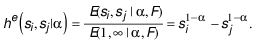
The aim of this sub-section is to illustrate basic facts on employment dynamics over the life cycle of establishments. It will begin by plotting data on the average number of employees per establishment as shown in Figure 2.1. The first thing to notice is that the average number of employees of plants in their first year is 2.4, which implies that Brazilian formal establishments are typically born small. One can also see that the average number of employees grows almost fivefold in the first 12 years of life (from 2.4 to 12), which corresponds to an average annual growth rate of 15.5%.
Source: Source: Authors’ estimations based on micro-data from RAIS.
Figure 2.1 also shows a great deal of heterogeneity across ages: in the second year the growth rate is very high (116%), then it decreases gradually reaching 4.5% in the 12th year. For future reference, it is worth pointing out that it takes about seven years for the typical establishment born in the Brazilian formal sector (that is, a plant that starts off in business with 2.4 employees) to reach the lower boundary of the range in size associated with middle-sized establishments (usually taken to be from 9 to 49 employees in the literature, as will be detailed later in this chapter).
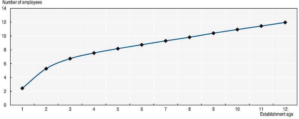
Such reference to the “typical” life cycle pattern of an establishment deserves two cautionary notes. First, as attested by Figure 2.A1.1 in Annex 2.A1, a great deal of heterogeneity can also be found across plants within the same age. Second, if the sample is divided into groups of plants according to their size at birth, as done in Figure 2.2, one can see that, on average, the group of smaller plants at birth does not reach the size of nine employees even at the 12th year in the formal sector.
Source: Source: Authors’ estimations based on micro-data from RAIS.
As an attempt to isolate the effect of age from other determinants of plant growth, such as the macro environment or cohort-specific conditions, this analysis performs Deaton and Paxson’s (1994) decomposition by age, cohort, and year (or macro) effects. The implementation is based on a regression model that uses dummies for ages, birth cohorts, and year of observation to explain the evolution of the establishments’ employment levels.2 The details of the method are outlined in Annex 2.A2. In principle, it would be possible to estimate cohort effects for every entry year of the establishments in the period of analysis of this study. However, for the decomposition exercise of this section, the choice was made to restrict the sample only to establishments that entered up until 2002 (inclusive). The advantage of doing this is that it guarantees that all plants in the sample can potentially reach at least 12 years of age between 1995 and 2013.
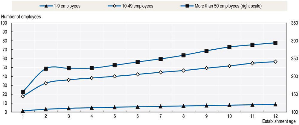
The results of the decomposition are reported in Figures 2.3and 2.4. Figure 2.3 shows that the age effect is remarkably similar to what this analysis has shown from raw data (Figure 2.1). After removing macro shocks and cohort-specific components, establishment size is an increasing function of age, displaying high growth rates in the initial years of life and a lower rate as establishments get older.
Note: Note: Normalised (age 1 effect = 0) age-dummy coefficients as specified in Deaton and Paxson (1994).
Source: Source: Authors’ estimations based on micro-data from RAIS.
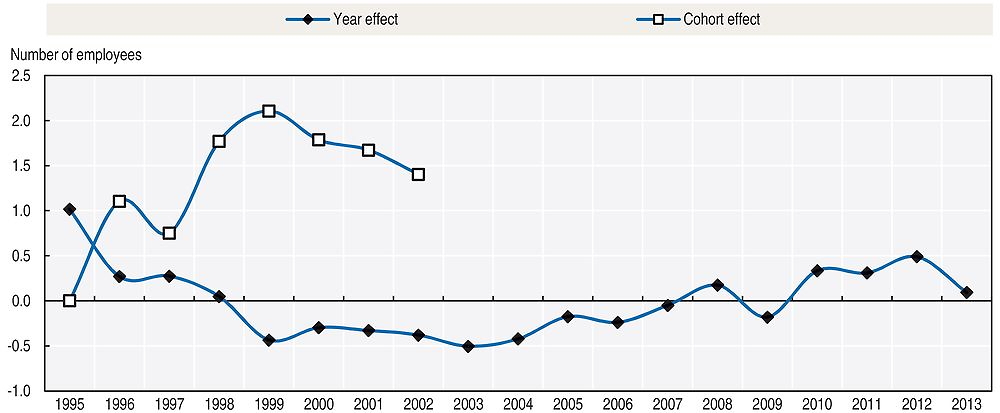
As for the other two components, Figure 2.4 shows that their magnitude is much smaller than for the age dimension. The year effects are similar to the pattern of economic growth in the period, while cohort effects depict an inverted U-shape peaking for the cohort born in 1999.3
Note: Note: Normalised (age 1 effect = 0) age-dummy coefficients as specified in Deaton and Paxson (1994).
Source: Source: Authors’ estimations based on micro-data from RAIS.
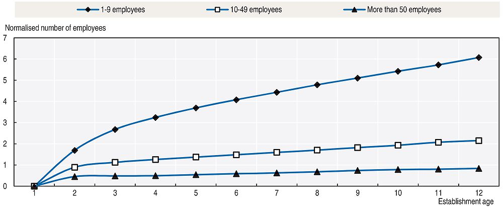
This study has also estimated the decomposition model for three different groups of the establishments at birth. The first group consists of establishments with less than nine employees (inclusive), the second by establishments with between nine and 49 employees (inclusive) and, the third by establishments with more than 49 employees. In order to facilitate the comparison across groups, the regression coefficients are divided by the average number of employees in each group when the establishments were born (1.3, 17.8 and 156.9, respectively). This study’s estimates, reported in Figure 2.5, reveal that the age effects are higher for the smallest group size, despite an increasing trend for all three groups. For instance, at age 12 the first group’s age effect alone would make the establishment grow 607%, while for the second and third groups, this number would be 215% and 84%, respectively. Despite the much higher age effect for the first group, the average plant born in this group (i.e. a plant born with 1.3 employees) does not surpass eight employees at the twelfth year of existence. Predicting the average size at that point of their life cycle, as a product of their initial size and the predicted growth rate for the first 12 years shown in Figure 2.4, would yield the predicted size of 7.89 (1.3*607% = 7.89). In other words, the pure age effect is not strong enough to transform a typical small plant into a middle-sized establishment.
Note: Note: Normalised (age 1 effect = 0) age-dummy coefficients as specified in Deaton and Paxson (1994).
Source: Source: Authors’ estimations based on micro-data from RAIS.
The composition effect due to establishment deaths
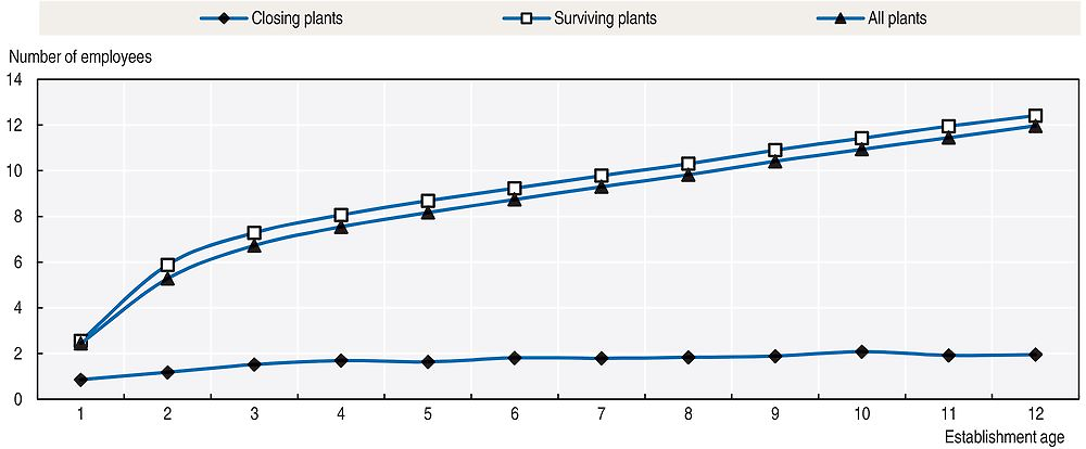
Apart from macro and cohort effects, the pattern of employment growth reported in Figure 2.1 may be affected by the process of establishment death. The observed pattern is reproduced by the line with triangular markers in Figure 2.6. The other two lines represent the average number of employees by age for two parts of the sample. For each age the sample is split into establishments that survive at least one more year (upper line) and establishments that appear for the last time in this study’s data at that age (lower line). These last two lines clearly show that the overall pattern is influenced by the death of plants. Indeed, there is a striking contrast between the average number of employees in the two partitions of the sample, and the difference increases with establishment age. In the first year the plants that survive are three times bigger than their non-surviving counterparts (closing plants), while in the twelfth year the average size of the two groups differs by a factor of nine.
Source: Source: Authors’ estimations based on micro-data from RAIS.
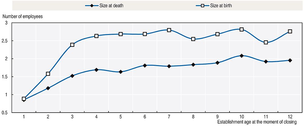
It is worth noticing that the average size of closing plants stays around one employee for all considered ages, indicating that a typical closing plant is very small at the moment of its death. Figure 2.7 reinforces this result by comparing the average size of closing plants at the moment of their death with the size of the same group of plants at birth. The results point to a lower average size at death than at birth for the same plants. This may partially explain why closing plants tend to be smaller than surviving ones, as shown in Figure 2.6.
Source: Source: Authors’ estimations based on micro-data from RAIS.
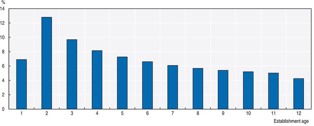
The fact that closing establishments tend to be small at birth and even smaller when they die generates a composition effect on the evolution of the overall average size. The (conditional on age) distribution of plants across sizes shifts towards bigger establishments when smaller plants close and leave the sample. This composition effect will be higher the larger the share of closing plants in the sample. Figure 2.8 shows the plant mortality rate by age (the proportion of establishments that die at a given age in relation to the total number of establishments with that age). One can see that this is a critical issue especially in the second (13%) and third (10%) years of plant life, a finding that is in line with evidence for other countries (see Calvino, Criscuolo and Menon, 2015). After the second year the mortality rate trend becomes negative, reaching 4% at age 12.
Source: Source: Authors’ estimations based on micro-data from RAIS.
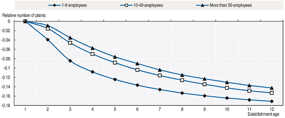
The pattern of mortality rate above can also be influenced by macro or cohort-specific shocks. Therefore the evolution of the number of establishments is also decomposed by cohort, time and age effects using the previous decomposition method. This exercise is done for the same three size groups previously used (i.e. establishments born with up to nine employees, above nine but less than 49 employees, and over 49 employees). Figure 2.9 shows the age effects, which are now normalised with respect to the number of establishments in each size class at age one.
Note: Note: Normalised (age 1 effect = 0) age-dummy coefficients as specified in Deaton and Paxson (1994).
Source: Source: Authors’ estimations based on micro-data from RAIS.
This study’s results point to negative (normalised) age effects, meaning that the number of establishments diminishes with age, and that their absolute values are higher for the smallest group size. For instance, at age three around 8% of plants that were born small (i.e. below nine employees) would die because of their age, whereas this figure for the middle and upper groups is around 4%. Although the age effect of the smallest class size gets closer to those of the others at higher ages, it is still higher (in absolute value) at age 12 (17% against 15%).
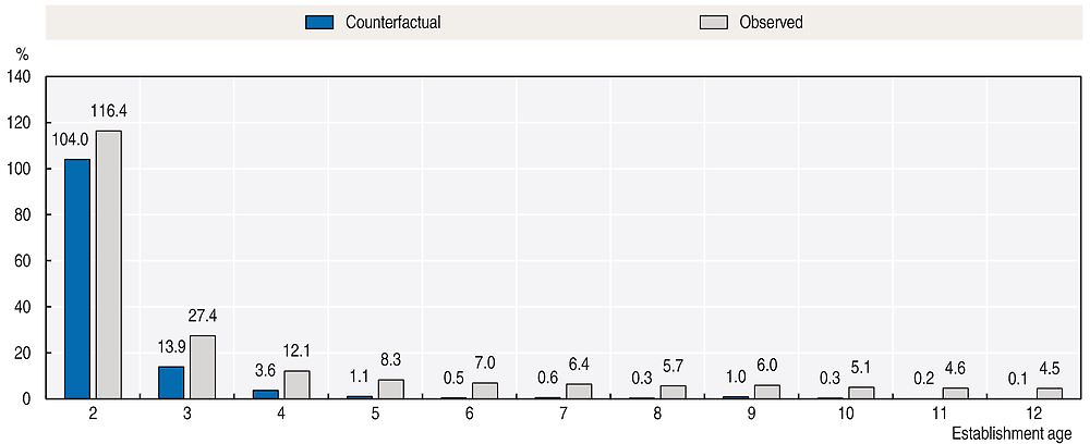
This study made an attempt to measure the importance of the composition effect. For this purpose two average employment growth rates were computed for each of two consecutive ages. One is the observed growth rate from Figure 2.1 and the other is a counterfactual growth rate that maintains in the sample also those plants that died in the age interval under consideration. Clearly, it is impossible to actually know the employment level of the dead plants had they survived one more year. It is likely that the number of employees would have diminished for a significant fraction of them, but it could also be that many would recover and even increase the size of their labour force. The choice was made to construct the counterfactual by imposing zero growth on dead plants, that is, for those plants the same employment level was imputed as in the year preceding death. Figure 2.10 reports the two employment growth rates by plant age.
Source: Source: Authors’ estimations based on micro-data from RAIS.
Figure 2.10 evinces that the composition effect is quite important, especially after the second year of life. For instance, in the second year, the counterfactual growth rate corresponds to a third of the observed rate and from the third year on the counterfactual rate is virtually zero. This comparison suggests that the observed growth rates for these ages were substantially influenced by the “cleansing” effect of plants’ death. One implication of this counterfactual exercise is that, without the death process, employment growth would be much weaker and the typical establishment born in the Brazilian formal sector would not reach the threshold of middle-sized establishments.
In sum, these results make it possible to draw a picture of the employment dynamics in the formal sector in Brazil with the following characteristics: a typical establishment is born small, grows relatively quickly in the first years but experiences a lower growth rate thereafter. Pure age effects have a much higher impact on the dynamics of employment growth than the macro and cohort effects and they display the same pattern across ages as that observed for a typical establishment. The results also show that plants which close down tend to be small and that a large percentage of establishments that are born small die before reaching the age of three. They further demonstrate that growth pattern of employment is affected by the death process of plants, producing a cleansing effect that arguably inflates the magnitude of the growth rate as age grows.
This analysis’ results clearly evince that the employment dynamics of small establishments in Brazil is quite different from that of larger plants. One may then speculate that if a large percentage of small establishments die early and the surviving ones do not grow very much, the establishment size distribution in Brazil is likely to display a lower concentration of middle-sized establishments. The following section will address this question.
The “missing middle” and establishment size distribution in Brazil
Tybout (2000) shows evidence of a much higher concentration of employment in small establishments in low-income countries than in industrialised countries. The evidence collected by Tybout (2000) also shows that the employment share of the middle part of the distribution was considerably lower in the former than in the latter group of countries.4 These results have been interpreted as evidence that small establishments have more difficulties in growing into mid-sized establishments in developing countries. The thinner middle part of the size distribution for this group of countries has been recognised by the field of development economics and baptised the “missing middle” phenomenon.
Many explanations have been proposed for the higher concentration of small establishments and the missing middle phenomenon in the developing world. A first group of explanations is based on institutional factors such as the regulatory and tax systems of developing countries. Since larger establishments have to cope with more intricate regulations, face higher labour costs (including the minimum wage and payroll taxes), and become more exposed to the enforcement of the law, many entrepreneurs prefer to be informal and remain small. As a response to some of these constraints, tax subsidy programmes have been introduced in many developing countries to stimulate small establishments to formalise their operations and grow in size. But even these initiatives have been criticised because they establish employment or revenue thresholds for tax exemptions that may end up discouraging small establishments from growing. The high licensing costs linked to launching an establishment, which are due to public sector inefficiencies (including corruption) can also hinder some talented but credit constrained entrepreneurs from starting their own businesses.
A second group of explanations is related to the insufficient development of financial markets and the high supply of unskilled labour that characterise low- and mid-income countries. Since poorly developed financial markets lack instruments to provide long-term finance, potential entrepreneurs and established small establishments find it difficult to obtain credit to invest in fixed capital or even to cope with cash flow problems. As a result, many small establishments are not born, do not increase their scale or even die. The relative trade closeness of those countries, e.g. because of high tariff and non-tariff barriers to trade, further hinders the access of small establishments to modern machinery, equipment, and technologies. Compounded with the obstacles to investment in modern fixed capital, the abundant supply of low-skilled labour pushes small establishments to start up and keep operating with labour-intensive, low productive technologies. The lack of supply of training in the basic skills to manage a small business is another factor that diminishes the chances of survival and growth of small enterprises in the developing world.
Another line of arguments has to do with the composition of demand. Most developing countries have a large percentage of low-income families whose consumption expenditure is concentrated on food items and basic goods that can be efficiently produced with small-scale, low-tech plants. This tends to create a production structure with low diversification, so many product and service markets are underdeveloped or missing. The low availability of wide, good-quality transportation networks is another factor that hampers the growth of small establishments. Lack of this type of public good increases costs and even deters investments to increase the scale of plants.
Despite the arguments for the existence of a missing middle, there are some concerns in the literature on whether it is in fact a characteristic of the establishment size distribution of developing countries. These concerns have been recently expressed by Hsieh and Olken (2014), who present a set of results using data from India, Mexico, and Indonesia that are not entirely compatible with the missing middle phenomenon. First, the authors show that the (average) productivity of establishments is positively related to their size, a finding that calls into question the common view that small establishments are the ones with high potential returns but that they do not to grow because they are somehow constrained (e.g. because of credit constraints). Second, they do not find evidence of kinks in establishment size or establishment revenue distributions around the thresholds established in the tax policy in those three countries. This implies that this type of tax policy does not seem to stop small establishments from growing. Finally, and more importantly for this study, they show that the histograms of establishment size distribution display a monotonic decay, a result that discards a bimodal pattern of high concentration of small and large establishments that would attest the presence of a missing middle.
To explain why the previous empirical literature had improperly established the existence of the missing middle (in terms of a presence of bimodality in the size distribution) in developing countries, Hsieh and Olken point to the combination of two issues associated with the use of the available data. The first is the incorrect use of the distribution of employment across plant sizes instead of the distribution of plant sizes. They argue that the theory is focused on the establishments’ decisions on whether or not to grow, so the relevant distribution for testing the existence of a missing middle is the distribution of plant sizes, not the distribution of employment. The second issue is that the results obtained in the literature are based on an arbitrary number of size bins (as well as the widths of these bins). Hsieh and Olken show that when the size of bins used in the literature (1-9, 10-49, and 50+ employees) is imposed to the establishment size distribution of India, Indonesia, and Mexico, the bimodal pattern that appears for the employment share distribution vanishes. Hsieh and Olken conclude that “the existing facts about the missing middle seem to come from the combination of these two transformations to the data: the transformation from the distribution of firms to the aggregate employment share, and the arbitrary binning of the employment share distribution” (p. 106).
To circumvent these criticisms, this analysis’ results are computed for the establishment size distribution and, for comparability with the results in Tybout (2014), also for the employment share distribution. Since the international evidence is only available for the manufacturing sector, the analysis is conducted separately for the entire formal sector and for the manufacturing sector alone. To deal with the problem of choosing an arbitrary number of size bins and their widths, this analysis also varies both dimensions.
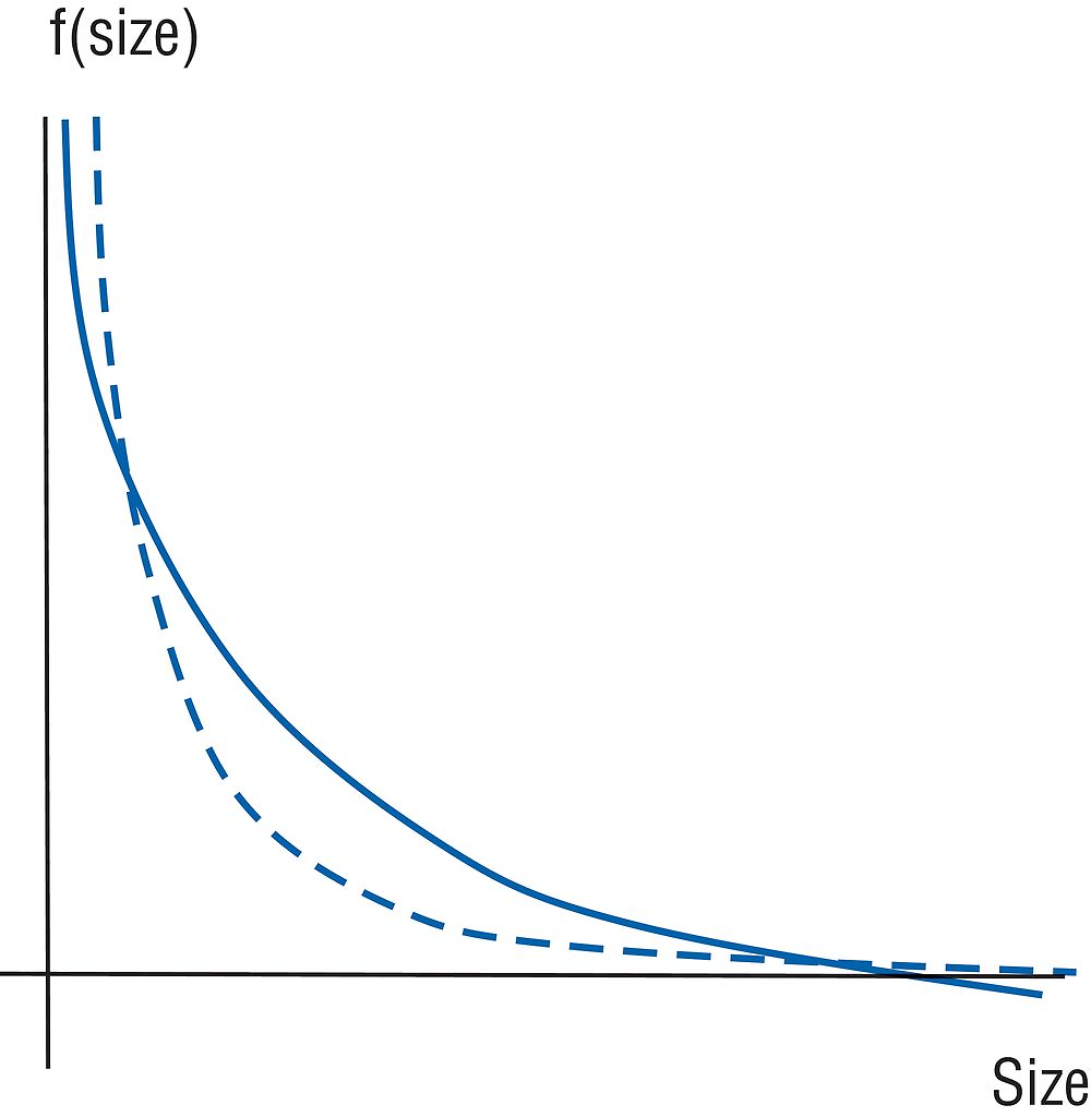
It is not considered that bimodality is the only criterion to evaluate the presence of a missing middle in the (establishment) size distribution. Indeed, the empirical distribution of a developing country can be unimodal and yet its middle part could be thinner than the corresponding middle part of the distribution of a developed country (e.g. the United States distribution). The hypothetical distributions displayed in Figure 2.11 – which is based on Tybout (2014, p.2) – shows this case, where the dashed line represents the density of establishments in the developing country and the solid line the density of establishments in the developed country. As the comparison of the two lines shows, though both distributions are unimodal, the share of mid-sized establishments in the developing country is smaller than the corresponding share for the developed one.
Source: Source: Authors’ analysis based on Tybout (2014), “The missing middle, revisited”, https://assets.aeaweb.org/assets/production/articles-attachments/jep/app/2804/28040235_app.pdf.
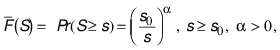
The main objective of this section is to analyse whether the establishment size distribution of the Brazilian formal sector displays a missing middle. This analysis follows Tybout (2014), who proposes a method that contrasts the observed shares of the establishment size distribution with the corresponding predicted shares of what is considered the best description of establishment size distributions in the literature: the Pareto distribution.5 The idea is that substantial differences between the theoretical and observed shares constitute evidence of under- or over-representation of the size groups. If the middle part (however defined) of the observed distribution is relatively under-represented, this is considered as evidence that there is a missing middle.
As in the previous section, the data only cover the formal sector in Brazil. Although the share of informal sector employment decreased markedly during the last decade, informal employment still represents around 20% of the labour force in the country. As informal establishments tend be small, this analysis’ results will probably understate their weight in the left tail of the establishment size distribution. As before, this study’s universe is the total set of establishments that belong to the private, non-agricultural sector in the Brazilian formal sector. To be compatible with the analysis of other parts of this study, this sample is formed by all establishments that were born from 1995 onwards. If this analysis computed its results only for establishments in their first years of existence, the size distribution would be too heavily influenced by the size profile of young establishments. Hence, the results are obtained using the last year available in this study’s data, 2013, for which the size distribution is more stable, as it becomes also influenced by the presence of older establishments. The main conclusions do not change when the exercise is implemented using the whole sample of establishments, and not only those observed in 2013.6
This study begins by showing histograms of the size distributions. Figure 2.12 presents the distribution of plant size while Figure 2.13 the distribution of employment shares by establishment size. Following Hsieh and Olken, it uses bins of ten workers up to size 200 and vary the lower cut-off of the range to make the shares more easily visible. It also shows a graph for sizes between 201 and 1 000 using bins of 50 workers and a graph for sizes over 1 001 employees with bins of different widths.
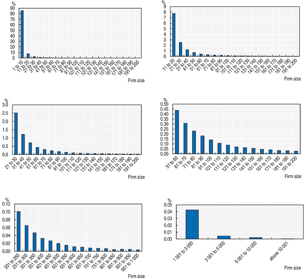
Note: Note: The sample is formed by all private, non-agricultural establishments born since 1995.
Source: Source: Authors’ estimations based on micro-data from RAIS.
Figure 2.12 reveals that the plant size distribution is highly right skewed displaying a very high concentration of small plants and a monotonic decline in the shares of larger establishments. This shape is similar to that presented in Hsieh and Olken for India, Indonesia, and Mexico. Although it is not considered that bimodality is the only criterion to check when deciding whether a distribution displays a missing middle, no evidence is found either of bimodality in the establishment size distribution for Brazil. Figure 2.13 shows that the employment share distribution is also right skewed, although the decline in shares is naturally smoother than for the plant size distribution. No bimodality is evinced in Panel 2 either. Though not shown, these findings are also valid for the manufacturing sector alone.
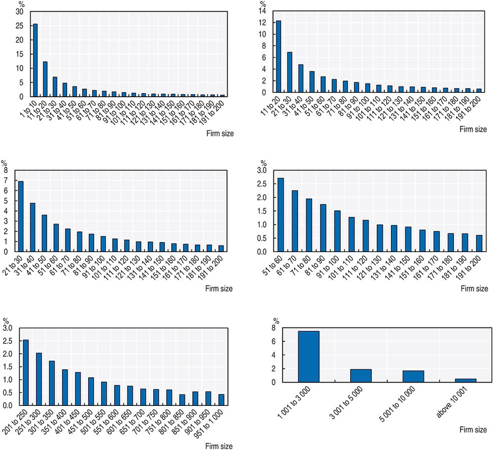
Note: Note: The sample is formed by all private, non-agricultural establishments that were born since 1995.
Source: Source: Authors’ estimations based on micro-data from RAIS.
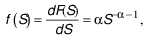
The Pareto distribution has been established as the best characterisation of establishment size distributions for developed countries.7 Following the method proposed by Tybout (2014), this study contrasts the empirical size distribution for Brazil with its closest theoretical Pareto distribution. The idea behind this procedure is that observed deviations between the shares of the predicted and the actual Pareto distributions indicate which parts of the empirical distribution are under or over-represented.
The upper tail of the Pareto size distribution can be written as:
 (1)
(1)
where S denotes establishment size, α is the shape
parameter, and s0 is the scale parameter that represents the
minimum possible value assumed by S. It is
assumed that the smallest plant employs one single worker, so s0 = 1. Larger values of α imply higher concentration
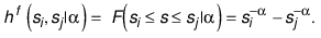
of smaller establishments in the size distribution. From (1), the share of
establishments (hf) in the size range  is given by:
 (2)
(2)
To calibrate the value
of α the main approach suggested by Tybout (2014) is used. The method searches
for the value of α that minimises the Euclidian distance between the log of
vector s of actual shares given by the
Pareto distribution and the log of vector  of predicted shares given by the empirical
distribution.8
of predicted shares given by the empirical
distribution.8
Since the bulk of the literature is based on the employment share distribution across plant sizes, this study also implements the method for this distribution. Given that the employment share in each bin can be obtained by multiplying the number of establishments in each bin with the average employment size of establishments in the bin, expression (2) can be written in terms of employment shares (he) as:9
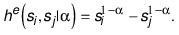 (3)
(3)
This analysis obtains results for different number of size categories and for different values of the cut-off points that define these categories. It initially defines three bins (called lower, middle, and upper) and varies the cut-off points to verify the sensitivity of the results to different widths of the bins. It employs the usual three bins that appear in the literature: 1 to 9, 10 to 49, and over 50 employees, but as shown in the tables below it uses various distinct cut-offs. Results are obtained for the plant size distribution (Table 2.1 for the entire formal sector and Table 2.2 only for the manufacturing sector) as well as for the employment share distribution (Table 2.3 for the entire formal sector and Table 2.4 only for the manufacturing sector). The second column in these tables reports the calibrated value of α that is retrieved by the method. Columns 3, 4, and 5 display the difference between the actual and predicted shares of the lower, middle, and upper categories respectively. The international evidence is only available for the employment share distribution in the manufacturing sector, so only Table 2.4 contains results that are comparable to those available in the literature. In Table 2.5 the number of bins is increased to six to see whether the results are sensitive to finer partitions of both the establishment size and the employment share distributions.
Table 2.1 presents the results for the plant size distribution for the whole formal sector. It reveals that there is excess concentration of small-sized establishments relatively to the benchmark Pareto distribution. In contrast, the middle size category is less populated than would be predicted by the Pareto distribution for all lower and upper bounds used to define the widths of the bins. As for the upper category, column 3 shows that its share is very close to that predicted by the Pareto. These pieces of evidence thus suggest that the missing middle phenomenon is observed for the Brazilian formal sector. Interestingly, the value of α is very close to one, suggesting that the upper tail of the distribution of establishment size in the formal sector in Brazil is almost exactly inversely related to the size of the establishments.
Table 2.2 reports the results for the manufacturing sector alone. Compared to the whole formal sector, the over-representation of small establishments is much higher and the under-representation of middle-sized establishments is much deeper. Larger establishments in this sector also appear to be under-represented but much less than the middle category. These figures also evince the presence of a missing middle in the establishment size distribution of the manufacturing sector in Brazil. As in the aggregate formal sector, the value of α is also very close to unity in the manufacturing sector.
The results for the employment share distribution across plant sizes for the formal sector are reported in Table 2.3. Contrary from what was observed in Table 2.1, here there is over-representation of both the smallest and largest categories. Naturally, the middle of the distribution is thinner than would be expected by the Pareto distribution, so the missing middle phenomenon is also apparent when the employment share distribution is used.
Table 2.4 contains the results for the employment share distribution only for establishments in the manufacturing sector. Similar to Table 2.3, there is overconcentration of employment in the lower and upper categories and a thinner middle part than predicted by the benchmark Pareto distribution. Table 1 in Tybout (2014), which is based on the 1-9, 10-49, and 50+ partition, reports that the negative gap for the middle category in the manufacturing sector is -0.084 for India (2011), -0.085 for Indonesia (2006), and -0.030 for Mexico (2006). The corresponding figure for Brazil is -0.139, so taking the employment share distribution as the reference for caparison purposes, the missing middle phenomenon seems to be slightly stronger in Brazil than in the Asian countries and considerably more severe than in Mexico.
In Table 2.5 the number of bins is doubled to six in order to verify whether the patterns of the previous tables are sensitive to way the distribution is partitioned. When using the establishment size distribution (Panel A), an under-representation of the middle part can also be seen, particularly in the second bin, whose upper cut-off is 29 workers (instead of the 49 threshold used before). This is valid for the entire formal sector as well as for the manufacturing sector alone. A similar pattern emerges for the employment share distribution (Panel B) but with the under-representation of the middle part being more spread across the central categories.
In sum, the method applied in this section shows an over-representation of small-sized establishments in the formal sector in Brazil. It also evinces that the middle part of the establishment size distribution is under-represented, with the upper part’s share corresponding to what would be expected by the Pareto distribution. Similar results apply when the employment share distribution is used. The result of a relatively thinner middle part provides support for the assertion that the missing middle phenomenon is also observed in Brazil.
Conclusions
This chapter’s results confirm that the middle part of the size distribution is “missing” in Brazil and apparently this feature is more intense than in other countries for which there are available results. This analysis of the dynamics of employment over the life cycle of establishments provides some clues on why there is a missing middle in the size distribution. Considering a representative establishment, the results show that it is born small (perhaps too small) and that the pattern of the growth rate over its life cycle imposes a long time span to surpass the threshold of a mid-sized plant.
These results also indicate that most of this life cycle pattern can actually be attributed to age effects, as the application of a novel decomposition method revealed a limited scope for potential confounding determinants such as the conditions prevailing at the time the plant was born (cohort effects) or the phase of the business cycle through which the plant existed (year effects).
Focusing on establishments that are actually born small, they start very small and, though the age effects are positive and high in their first years of life, they are not strong enough to transform them into plants of middle size. In addition, their mortality rate is quite high, especially within the first three years of their lives.
As in many other countries, the segment of micro and small establishments has received a great deal of attention from public policy in Brazil. Indeed, a myriad of programmes specifically targeted to this segment have been implemented by the national, state, and municipal spheres of government over the last decades. The number of initiatives and their specificities are too extensive to fit in this chapter but among the most important ones are an ample set of national and regional programmes that provide credit at low interest rates and credit guarantees to micro and small establishments, a wide programme that concedes tax subsidies for establishments whose revenues are below a defined threshold, a large programme of government procurement targeted to micro and small establishments, and a broad supply chain of training courses and technical assistance dedicated to help potential entrepreneurs and already established small businesses to improve their operation. As claimed by Nogueira (2016), Brazil is certainly the Latin American country with the largest and most diversified institutional framework to support this type of establishments.
Unfortunately, the effectiveness of these interventions has not been assessed, so it is difficult to say whether and to what extent they have actually affected the performance of the micro and small establishments in the country. Although this chapter’s results indicate that the performance of small establishments in the country is relatively poor, it is possible that the situation would be even worse had these programmes not been in place. Nevertheless, they clearly need to be redesigned, in particular towards increasing the articulation of the various initiatives within and between the three spheres of government.
References
Audrescht, D. and J. Mata (1995), “The post-entry performance of firms: Introduction”, International Journal of Industrial Organization, Vol. 13, Issue 4, pp. 413-419, https://doi.org/10.1016/0167-7187(95)00497-1.
Axtell, R.L. (2001), “Zipft Distribution of US Firm Sizes”, Science, Vol. 293, pp. 1818-1820, www.uvm.edu/pdodds/files/papers/others/2001/axtell2001a.pdf.
Calvino, F., C. Criscuolo and C. Menon (2015), “Cross-country evidence on start-up dynamics”, OECD Science, Technology and Industry Working Papers, No. 2015/06, OECD Publishing, Paris, https://doi.org/10.1787/5jrxtkb9mxtb-en.
Caves, R. (1998), “Industrial Organization and New Findings on the Turnover and Mobility of Firms”, Journal of Economic Literature, Vol. 36, No. 4, pp. 1947-1982, www.jstor.org/stable/2565044.
Deaton, A. and C. Paxson (1994), “Saving, Growth and Aging in Taiwan”, in Wise, D. (ed.), Studies in the economics of aging, University of Chicago Press, Chicago, www.nber.org/chapters/c7349.pdf.
Decker, R. et al. (2014), “The Role of Entrepreneurship in US Job Creation and Economic Dynamism”, Journal of Economic Perspectives, Vol. 28, pp. 3-24, http://econweb.umd.edu/~haltiwan/JEP_DHJM.pdf.
Haltiwanger, J., R. Jarmin and J. Miranda (2013), “Who Creates Jobs? Small versus Large versus Young”, The Review of Economics and Statistics, Vol. 95, pp. 347-361, http://econweb.umd.edu/~haltiwan/size_age_paper_R&R_Aug_16_2011.pdf.
Hsieh, C.-T. and B.A. Olken (2014), “The Missing ’Missing Middle’”, Journal of Economic Perspectives, Vol. 28, pp. 89-108, http://faculty.chicagobooth.edu/chang-tai.hsieh/research/missingmiddle.pdf.
Jovanovic, B. (1982), “Selection and the Evolution of Industry”, Econometrica, Vol. 50, Issue 3, pp. 649-670, www.jstor.org/stable/1912606.
Leidholm, C. and D. Mead (1987), Small-Scale Industries in Developing Countries: Empirical Evidence and Policy Implications, MSU International Development Paper No. 9, Department of Agricultural Economics, Michigan State University, Michigan, http://fsg.afre.msu.edu/papers/older/idp9.pdf.
Luttmer, E.G.T. (2007), “Selection, Growth, and the Size Distribution of Firms”, Quarterly Journal of Economics, Vol. 122, Issue 3, pp. 1103-1114, http://qje.oxfordjournals.org/content/122/3/1103.full.pdf.
Nelson, R. and S. Winter (1982), An Evolutionary Theory of Economic Change, Harvard University Press, Cambridge, MA, http://inctpped.ie.ufrj.br/spiderweb/pdf_2/Dosi_1_An_evolutionary-theory-of_economic_ change.pdf.
Nogueira, M.O. (2016), “O panorama das políticas públicas federais brasileiras voltadas para as empresas de pequeno porte”, IPEA, Brasilia, www.ipea.gov.br/portal/images/stories/PDFs/TDs/td_2217.pdf.
Tybout, J. (2014), “The Missing Middle, Revisited”, https://assets.aeaweb.org/assets/production/articles-attachments/jep/app/2804/28040235_app.pdf.
Tybout, J. (2000), “Manufacturing Firms in Developing Countries: How Well They Do, and Why?”, Journal of Economic Literature, Vol. 38, No. 1, pp. 11-44, www.aeaweb.org/articles?id=10.1257/jel.38.1.11.
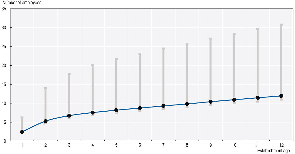
Note: Note: The vertical grey lines represent the interval between P10 and P90 for the size distribution conditioned at the age displayed at the horizontal axis.
Source: Source: Authors’ estimations based on micro-data from RAIS.
The estimated model is the following:
 (1)
(1)
where averagesize is a column vector of the average number of employees of establishments with m rows (where m is equal to the product of the number of cohorts, ages, and years), (age1,…,age19) are column vectors of age dummies, (cohort1995,…,cohort2002) are column vectors of cohort dummies and (year1995,…,year2013) are column vectors of year dummies.
The model (1) cannot be estimated due perfect collinearity since the cohort is a linear combination of year and age:
 (2)
(2)
In order to estimate model (1), Deaton proposes a normalisation that is based on the assumption that year effects capture cyclical fluctuations that have mean zero in the long run. This assumption makes the year effects orthogonal to a time-trend:
 (3)
(3)
where sy is an arithmetic sequence {0,1,2,3;..}.
Under assumption (3), Deaton and Paxson (1994) suggest estimating the model (1) by regressing the response vector on cohort dummies (omitting the first cohort), age dummies (omitting the first age) and a set of T-2 years dummies, defined as follows:
yeart*= yeart – [(t-1995)year1996 – (t-1996)year1995] for every t=1997,...,2013. (4)
The coefficients of the yeart* dummies give the coefficients of (year1997,…,year2013), the coefficients of (year1995 and year1996) can be recovered by conditions (4) and from the fact that all year effects add up to zero.
Notes
← 1. There are incentives for truthful reporting since the main purpose of RAIS is to administer a federal wage supplement (Abono Salarial) to formal sector workers.
← 2. This was originally proposed for the analysis of wages or consumption but can be applied to any other variable affected by these three dimensions.
← 3. As previously mentioned, all the establishments of cohorts after 2002 are excluded.
← 4. The evidence presented in Tybout (2000, Table 2.1) was gathered from different studies, in particular from Leidholm and Mead (1987). Most of the figures were only available for three bins of the employment share distribution, namely: 1-9, 10-49, and 50+ employees.
← 5. See Axtell (2001) and Luttmer (2007).
← 6. The results are available from the authors upon request.
← 7. Specifically, the Zipf distribution, a special case of the Pareto, is considered the best description of the firm size distribution. See Axtell (2001).
← 8. An alternative method suggested by Tybout (2014) chooses α so that the share of the smallest size category of the actual and predicted distributions matches exactly. This study also implemented this method and, although not shown, the results were qualitatively similar. Since the mean of the Pareto distribution is only defined for values of α higher than unity, it imposed this constraint in the estimation.
← 9. Letting F be the total number of establishments and using the density of the establishment size distribution:
total employment in the economy is given by:
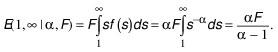
Total
employment in the size range  is
is
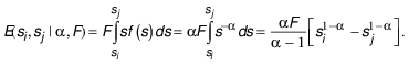
Thus,