Chapter 3. Understanding rural economies1
This chapter first considers the definition of “rural”, with a discussion of the characteristics of low-density economies and methods to capture some of those characteristics in the definition of rural regions. The second part of the chapter analyses key trends in rural regions, including trends in productivity, gross domestic product, employment, and demographic change, using the OECD extended typology that allows for the classification of rural regions according to their proximity to cities. There is a focus on the role of the tradable sector for productivity performance and the resilience of rural regions to the effects of the recent crisis.
-
Rural regions are diverse and highly influenced by their specific natural environments. Their development path is substantially different from the standard urban model. Certain rural regions in OECD countries have been highly successful in terms of economic performance and quality of life. Other rural regions have been less successful. The success or weakness of rural regions is considerably more affected by changes in economic conditions than in urban areas.
-
Rural regions employ different development models adapted to reflect specific features of having a low density of population and economic activity. This variability calls for a typology of different definitions of rural, such as: i) rural areas inside functional urban areas; ii) rural areas adjacent to functional urban areas; and iii) rural areas that are far from functional urban areas, i.e. “remote”.
-
There are different development patterns observed depending on the type of rural region. Rural regions close to cities are more dynamic than rural remote regions and also more resilient, displaying an economic performance similar to urban regions. Rural regions close to cities registered an average annual productivity growth of 2.15% in the period 2000-07 – higher than any other type of region.
-
Productivity growth in rural regions in the pre-crisis period was mostly accompanied by employment growth. Among those rural regions that experienced positive productivity growth in the period 2000-07, two-thirds also recorded positive employment growth. Since the crisis this pattern has been difficult to maintain.
-
Remote rural regions are particularly vulnerable to global shocks. Following the financial crisis, their average productivity declined by 0.61% per annum over the period 2008-12. This average hides the fact that some remote rural regions continued to perform well during and after the financial crisis.
Introduction
Rural regions are home to more than one-quarter of the OECD population and they contain the vast majority of the land, water and other natural resources in OECD countries. In a green growth context, they will be critical for developing a new type of economy. While rural regions have a reputation for being laggards in the growth process, as was shown in Chapter 1, this is not the case. In fact, Figure 1.8 shows that a considerable share of the 50 regions with the highest productivity growth in the OECD are mostly rural, which means that their high rate of growth took place in the absence of a large metropolitan centre. Moreover, while rural regions are individually small in terms of their level of regional gross domestic product (GDP), they collectively make a significant contribution to national GDP.
Improving our understanding of how rural regions contribute to national economies is the main goal of this chapter. The two main questions raised in Chapter 1 about falling rates of productivity and unequal regional growth have a clear rural dimension. While rural regions are increasingly, and more broadly, linked to urban regions – through markets, the movement of people, multi-level governance, the flow of environmental services and a variety of other ways – they have a distinct growth dynamic that is different from the urban model of growth. While rural regions rely on urban regions as the source of many of the goods and services they consume and as markets for much of what they produce, their economies reflect the special features of what can be called a “low-density economy”.
Low-density economies are typically characterised by several features. They include: a small local workforce that both limits the number and size of firms that can efficiently operate; a high reliance on the extraction and first stage processing of local natural resources that are then exported far beyond the region; sensitivity to transport costs; the possibility of strong competition with regions with similar economic structures; a reliance on innovations developed elsewhere as well as local innovator/entrepreneurs; and a local economy that is highly sensitive to regional, national and global business cycles (see also Chapter 1). Under favourable circumstances these economies can: demonstrate high levels of worker productivity; benefit from large inflows of capital that lead to increases in employment and productivity; and provide high wages and employment opportunities that contribute to a good quality of life for local households. Under unfavourable circumstances, such as low commodity prices, the rise of strong competitors, or resource depletion, rural regions can experience high rates of unemployment, population outflows and a deteriorating quality of life, both in terms of income and access to services.
The diverse situation of rural regions in the OECD is examined using data at a lower level of aggregation than was generally used in the first two chapters. The large regions (TL2) correspond to the highest subnational unit of governance – such as a state in the United States or a Land in Germany. These units typically contain multiple cities of varying sizes and a wide spectrum of different types of rural areas. In contrast, small regions (TL3) are a lower level of aggregation, such as a province in Belgium, an aggregation of counties into economic areas in the United States or regions in Finland (see the Reader’s Guide). While they still contain urban and rural territory, TL3 regions tend to be more homogeneous than TL2 regions. This allows for a more precise picture of the types of rural regions across a country and provides a basis for a better understanding of how differences in rural economic development have occurred in recent times within, and across, OECD countries.
Rural areas as places of opportunity
Rural areas provide traditional resources but they are increasingly providing vital new functions that use their resource base in novel ways. The role of rural regions as producers is well understood. Forestry, mining, oil, gas, electricity production, fishing and agriculture are almost exclusively rural industries. Much manufacturing also takes place in rural areas, in particular the first stage processing of natural resources. However, rural areas are more than just producers. They are more than “hewers of wood and drawers of water”. In recent decades, rural areas have experienced a fundamental transformation from places concerned with only resource extraction for export to places that are also concerned with local or direct use of resources, albeit without their direct consumption. These expanding rural activities include: various types of rural tourism, the preservation of wildlife and cultural heritage sites, the production of renewable energy, and the recognition of the key role that the rural environment plays in eco-system services, such as carbon capture or filtering contaminants from air and water.
These functions offer a new economic base for a rural region that can provide sources of income and employment beyond traditional activities. In many cases these functions are found in rural regions that are in close proximity to a large metropolitan centre. Proximity allows urban residents easy access to the rural region and the possibility of frequent trips within a year. In other cases, a unique high value resource may be found in a remote rural region that can only be reached with a large outlay on travel, making a visit an expensive proposition. Such activities might include: skiing in the Patagonia region of Chile; snorkelling in the Great Barrier Reef in Australia; observing the Saami people and their reindeer in Lapland in Finland; or producing solar power in desert areas of Arizona (United States).
Proximity to an urban region is an important predictor of rural growth. Rural growth does not only occur in rural regions that are close to cities, but proximity allows stronger linkages between urban and rural places that are increasingly important factors in understanding differences in rural growth. Two-way flows of many kinds are easier when urban and rural are adjacent (OECD, 2013). Urban residents have easier access to the green space of the countryside, while rural residents have easier access to advanced public and private services that are only found in cities. Indeed, the vast majority of rural residents and rural economic activity are found in close proximity to (functional) urban areas. While these urban and rural places are connected and interdependent, they remain distinct entities in terms of their economic functions, settlement patterns and ways of life. By contrast, in remote rural places there are fewer direct connections with cities and local residents and firms must rely almost exclusively on local providers of goods and services.
Restoring productivity growth is important in all regions, but especially in rural regions. Falling rates of productivity growth and concentration of growth in a few regions is a central problem for OECD countries in general, but often it is a crucial issue for their rural regions. Across the OECD, in almost all rural regions, the workforce is getting older and smaller. Youth outmigration is typically at a high level, and the average level of formal education and worker skills is lower than is the case in urban areas. These workforce issues have important implications for rural economic development. In a future with fewer workers economic growth must come from higher productivity. Without a strong workforce the presence of a strong natural resource base will not be enough to ensure economic prosperity. Moreover, it is generally recognised that infrastructure investments are required in rural regions to improve connectivity to urban markets. However, investments that will improve human capital are perhaps more important, because without a workforce with adequate skills, firms in rural regions may be unable to maintain production as local workers age and retire.
The 2007-08 crisis provides an example of how rural regions are impacted by external shocks. That crisis presented a major challenge to OECD economies, including their rural areas. Although many rural areas suffered less in terms of direct job loss than urban regions, due to the nature of their economies, the crisis put major pressure on public spending in virtually all rural regions. The budget constraints of national and regional governments led to reduced subsidies for rural regions that could not be offset with local revenue. The result was reduced access to public services and pressure to find new ways to deliver services in rural areas. Even after a partial recovery, these budget pressures continue and are exacerbated by higher demands in rural regions as local populations age, and economies that were once strong are impacted by recent declines in global commodity prices.
Support from national governments is important for the small and specialised economies found in rural regions. OECD member governments have had a longstanding commitment to supporting their rural residents. Traditionally this support focused on agriculture and a few other resource industries, as these provided the majority of rural income and employment. Now, as rural economies diversify and rural economic development follows multiple paths, a more nuanced form of support is needed. The OECD New Rural Paradigm (OECD, 2006) was a first step in offering a framework for a broader perspective on how countries could better support rural residents in their development efforts. Since its publication, conditions in rural areas have evolved due to the ageing of rural populations, changing demands for natural resources, an increased concern with climate change and greater fiscal limitations in government budgets.
An updated rural policy framework should reflect both new conditions for rural regions and a more advanced understanding of rural economies. Chapter 4 provides a discussion of how OECD member countries have designed and implemented useful rural policies and of a new framework for integrating these policies into a general delivery mechanism. This new framework – Rural Policy 3.0 – reflects the evolution of rural economies since 2006 and the continuous efforts to better understand how national governments can best support them in their efforts to develop.
Defining rural regions
Recent definitions of rural regions recognise that there are many kinds of rural areas. While the OECD has developed a specific definition with a focus on international comparability, individual countries continue to explore alternative definitions that can better suit their particular needs. Importantly, the OECD definition informs the OECD Regional Database (OECD, 2015a) which is used to analyse the performance of the different types of rural region below.
New approaches to understanding how rural spatial dynamics underpin the OECD rural definitions
There is no internationally recognised definition of a “rural area” and there are ongoing debates about how best to define the concept. While a low population density is a common starting point, it is generally recognised that “rurality” is a multi-dimensional concept, which can embody different meanings for different purposes. For example, as a geographical or spatial concept, a socio-economic or socio-cultural descriptor, a functional concept related to, for instance, labour market flows, or simply as “not urban”. One way to understand rural is through identifying differences in rural and urban linkages as a function of the distance of a rural place from an urban agglomeration.
Urban and rural areas are interconnected through different types of linkages that often cross traditional administrative boundaries. These interactions can involve: demographic, labour market, public service and environmental considerations. They are not limited to city-centred local labour market flows and include bi-directional relationships with rural-urban functional linkages (Figure 3.1). Each type of interaction encompasses a different geography forming a “functional region”.
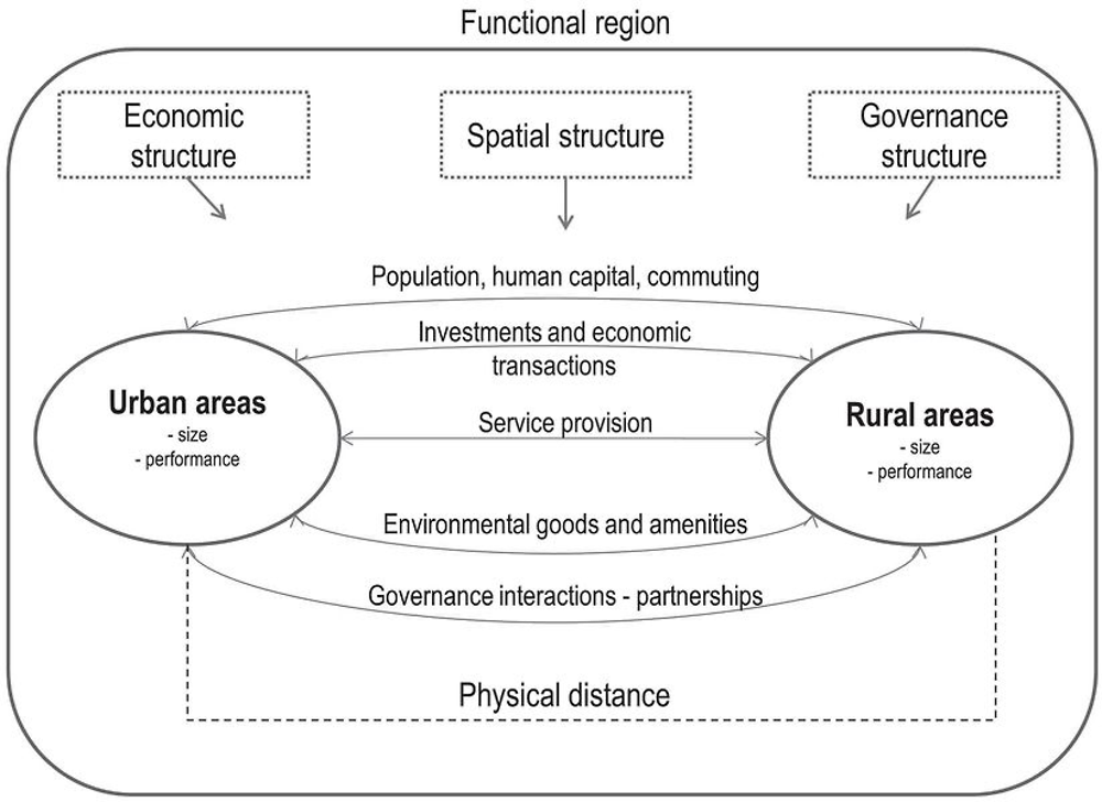
Source: OECD (2013), Rural-Urban Partnerships: An Integrated Approach to Economic Development, https://doi.org/10.1787/9789264204812-en.
The complexity of the relationships can be represented along an urban to rural continuum from more to less densely populated areas and gradations in between. While there are no sudden breaks in these spatial relationships, there is great diversity in the size and types of interconnections. Figure 3.2 further illustrates the concept. It depicts a distribution of urban (large dots) and rural (small dots) areas scattered through space showing a continuum of settlement patterns based on location, proximity and density characteristics. Such spatial distinctions can yield important insights for public policy, because the range of opportunities and constraints facing any particular place vary with its location, and this has implications for jobs, services and infrastructure development, among other considerations.

Note: The size of dots indicates relative population size. Large blue dots represent urban settlements and small light blue dots rural settlements.
In developing definitions of “rural”, the unit of analysis plays an important role. There is a choice between a functional unit, based on observed behaviour, and an administrative unit, based on political boundaries. Functional definitions better capture complex economic flows and interactions between highly linked urban and rural places. Conversely, administrative units are better suited for the design and delivery of public services and managing public administration.
The three types of rural regions in the OECD approach have different degrees of linkage with metropolitan areas
Building on the potential degree of interaction between rural and urban areas to classify rural regions, a three-category typology has been developed. There are: i) rural areas within a functional urban area (FUA); ii) rural regions close to a FUA; and, iii) remote rural regions (Figure 3.3). Each type has distinct characteristics, challenges and policy needs:
-
Rural areas within a FUA – these types of rural areas are an integral part of the commuting zone of the urban centre and their development is fully integrated within a FUA.
-
Rural regions close to a FUA – these regions have strong linkages to a nearby FUA, but are not part of its labour market. There are flows of goods, environmental services and other economic transactions between them. While the urban and regional economies are not integrated, much of the growth in the rural region is connected to the growth of the FUA. The majority of the rural population in OECD countries lives in this type of rural region.
-
Remote rural regions – these regions are distant from a FUA. Connections to FUAs largely come through market exchange of goods and services, and there are only limited and infrequent personal interactions outside the rural region, but there are good connections within the region. The local economy depends to a great extent on exporting the output of the primary activities of the area (see the discussion on “low-density economies” below). Growth comes from building upon areas of absolute and comparative advantage, improving connectivity to export markets, matching skills to areas of comparative advantage and improving the provision of essential services (e.g. tourism).

Note: The circle delimits a FUA; the blue hexagon represents the most urbanised part of the FUA, while the small light blue dots represent rural communities
Because they are structurally different, the three types of rural region face different development challenges
Understanding the common challenges and opportunities within each of the three categories leads to the possibility for shared action and more effectively targeted policy responses. Table 3.1 summarises these challenges and opportunities.
-
For rural areas within the commuting zone of a FUA, development is intimately linked to that of the core city. The main challenges facing this type of rural region are: service delivery, as services concentrate in the core area; the matching of skills to the requirements of the labour market; and managing land-use policy brought on by increasing pressures of the urban core.
-
Rural areas that are close to FUAs often enjoy a good industrial mix, which makes their local economies more resilient. They are also frequently able to attract new residents. The economic and social diversity of rural areas that are close to a FUA can pose challenges such as competition for land and landscape in the case of economic activities, and different needs and visions between old and new residents. Conflicts over development patterns can occur between these regions and the nearby FUA.
-
For remote rural regions with a relatively dense settlement pattern primary activities play a relevant role in the regional economy. Growth comes from building upon areas of absolute and comparative advantage, improving connectivity to export markets, matching skills to areas of comparative advantage and improving the provision of essential services. A strong resource base can result in high levels of income and productivity, but it can also result in cyclical (boom-bust) economies. These regions can face challenges in retaining and attracting workers and tend to have weak service delivery mechanisms.
OECD countries have adopted rural definitions that reflect their specific needs and have evolved over time
Since context and geography matter, it is no surprise that OECD member countries have adopted a wide range of definitions delimiting urban and rural borders. Indeed there is no such thing as an optimal or universally agreed upon rural definition for implementing policy. The wide diversity of rural definitions (Table 3.A3.1 in the Annex) also reflects different criteria that exist to elaborate definitions including density, economic activity, size or distance to services, among others.
Countries are trying to move away from traditional definitions of rural areas as simply the remaining “left over” space that is not urban. Traditional definitions do not differentiate among different types of rural areas or do not recognise areas of strong urban and rural interactions. With the advancement of Geographic Information System (GIS) tools and better availability of data, many OECD countries have revised and advanced their definitions to incorporate new criteria such as distance and accessibility to services, and are now recognising areas with strong urban and rural interactions. The shared goal in these efforts is to have a tool that can more accurately delimit rural areas and identify common challenges and opportunities to design better policy responses.
A number of countries are adopting new definitions and making use of a wider range of data sources including commuting, labour market or transportation network data. For example, Austria and Spain mainly use the urban-rural typology of the European Union (EU)2, New Zealand has adopted a definition that distinguishes between rural areas with high, moderate or low urban influence and those deemed rural-remote by drawing on both population density, place of employment and commuting data (Statistics New Zealand, 2016).
Italy has developed a definition based on service accessibility and policy objectives. Rural areas in Italy are distinguished from urban poles and split into three categories: intensively cultivated and plain areas, intermediate rural areas and finally, areas with lagging development. This classification is based on population density indicators and share of agricultural land.3 Italy has also adopted a classification of rural areas based on policy objectives. In Italy, “Inner Areas” are groups of municipalities characterised by “inadequate access to essential services.” This classification is driven by policy purposes: by measuring access to health care, education, and transportation, policies can be specifically designed to meet local needs. Inner Areas are those further than 75 minutes driving time away from “Service Centres”, which are municipalities that have an exhaustive range of secondary schools, at least one highly specialised hospital, and a railway station. All Italian municipalities have been classified according to the distance (travel time) from these Service Centres.
France is also advancing on a definition considering accessibility, but with a different methodology. In France, the National Institute of Statistics and Economic Studies has developed an indicator that examines the accessibility of services and amenities that are important to daily life for communities of varying population densities (INSEE, 2016). The indicator distinguishes between densely populated towns, intermediately populated towns, sparsely populated municipalities and very sparsely populated municipalities. It further considers access to: health, education and social services; sport, leisure, tourism and cultural amenities; and shops for food, goods and services. Taken together, the indicator helps policy makers better understand and act on regional differences in service accessibility.
In some countries, revised rural definitions have been spurred on by the reform of local governments. Finland is a case in point. The country first introduced a rural typology in 1993 based on municipal boundaries. It identified three rural types: i) rural areas close to urban areas; ii) rural heartland areas; and iii) sparsely populated rural areas. Started in 2005, a restructuring of municipalities resulted in fewer and larger municipalities and an increasing degree of rurality within municipalities. Consequently a new rural typology was needed in order to better capture these dynamics. Statistics based on administrative boundaries were found to be unsuitable for spatial analysis because they could not adequately represent regional differences. To this end, Finland has adopted a classification based on spatial data sets and on seven regional types: inner urban area, outer urban area, peri-urban area, local centres in rural areas, rural areas close to urban areas, rural heartland areas and sparsely populated rural areas. The framework employs a wide range of variables to capture the diversity of rural places including: population, employment, commuting patterns, construction rates, transport access and land use data. Collectively these variables are used to construct indicators of economic activity, demographic change, accessibility, intensity of land use and other attributes for each region.
Rural definitions are important and can have political, economic and social consequences
In summary, there is no single and best way to define rural regions across OECD countries. There are, however, emerging best practices that should be taken into account:
-
A single category of “rural” misses the diverse rural realities. Definitions that only consider the characteristics of urban areas and, by default, define the remaining territory as rural areas are ill-equipped to capture the realities of modern rural economies that are often based on strong interrelations with urban areas, changing commuting patterns and accessibility to external markets.
-
Definitions should capture rural-urban linkages. The recognition of mixed spaces is important. Definitions recognising areas with strong urban and rural interactions have the potential to better build on synergies and complementarities between urban and rural areas.
-
Administrative definitions that impose large minimum populations may lead to undesirable outcomes. Efforts to create a rural region that has a big enough population to meet minimum scale requirements for public service delivery can be counterproductive. In rural areas with low population density, large schools may seem to offer more classroom options, but impose high transport costs. Similarly, consolidating rural local governments to reduce administrative costs may lead to residents losing any connection to their representative and facing high costs in accessing public services. Considerations of distance and accessibility are very important for low-density areas. In adopting rural definitions, governments need to consider the implications for social cohesion within a space or geography (e.g. the desire for people to be connected to one another and have shared community visions) along with the delivery of services. The two may be inversely related – larger service-delivery regions may be desirable for the sake of cost effectiveness, but could negatively affect social cohesion by binding together communities that in fact have little in common.
Definitions of rural areas have important implications for the delivery of services and allocation of public resources. Chile is an illustrative case in this regard. The OECD Rural Policy Review of Chile (OECD, 2014a) found that the country was using a rural definition that classified even the smallest settlements into the “urban” category. As a result, only 12% of Chile’s territory was identified as rural, with the remaining 88% classed as urban. These results were inconsistent with the observed distribution of the population and with the vast contribution of rural industries such as mining, agriculture and forestry to GDP and exports (OECD, 2014a). The definition also created the impression that rural development was only a minor issue and had implications only for the delivery of services and support to rural areas. As a result of this analysis, Chile is presently reviewing its rural definition to better capture these dynamics.
A new narrative is needed to clarify that rural regions make important contributions to national objectives, including economic development and prosperity. As seen in the case of Chile, the use of definitions is critical in contributing to this new narrative. By using outdated definitions, rural Chile is depicted as lagging, poor and remote. With a revised definition, a different picture emerges: rural areas are dynamic and poverty is mainly associated with mixed peri-urban areas.
The OECD regional typology
Country definitions are adapted to their specific needs and are mainly used for policy implementation, while the OECD has developed a definition to allow for international comparisons. The OECD first developed in 1991 a regional typology using a simple and commonly accepted criterion rule to define rural regions. This definition has been widely used to compare trends and patterns among OECD member countries, and will be used for the analysis of this chapter. The OECD regional typology incorporates some of the criteria used by individual OECD countries to define regions (e.g. mixed, different types of rural regions, cohesion), but it aims to develop a comparable definition for the purpose of analysis and therefore applies the same criteria across all OECD countries. International comparability requires some concessions compared to the typology outlined above. The typology is used to classify OECD TL3 regions, distinguishing predominantly urban (PU) regions from intermediate (IN) and predominantly rural (PR) regions (Box 3.1). An extended typology further classifies predominantly rural regions into regions that are “predominantly rural close to cities” and those that are “predominantly rural remote”. This captures two of the types of rural areas outlined above (Table 3.1). Ideally the typology would also be able to identify rural areas inside functional urban areas, but this is not feasible at the TL3 level and would require data at smaller regional scales.
The OECD regional typology is part of a territorial scheme for collecting internationally comparable “rural” data. The OECD typology classifies TL3 regions as predominantly urban, predominantly rural and intermediate. This typology, based on the percentage of regional population living in rural or urban communities, allows for meaningful comparisons among regions of the same type and level. However, there is a trade-off: along with the benefits of international comparability, this framework necessarily has the drawback of not being as precise as the more refined definitions that are used to deliver policies in some countries.
The OECD regional typology
The OECD regional typology is based on three steps. The first identifies rural communities according to population density. A community is defined as rural if its population density is below 150 inhabitants per km² (500 inhabitants for Japan to account for the fact that its national population exceeds 300 inhabitants per km²). The second step classifies regions according to the percentage of the population living in rural communities. Thus, a TL3 region is classified as: predominantly rural, if more than 50% of its population lives in rural communities; predominantly urban, if less than 15% of the population lives in rural communities; and intermediate for values in between.
The third step is based on the size of the urban centres. Accordingly, a region that would be classified as “predominantly rural” in the second step is classified as “intermediate” if it has an urban centre of more than 200 000 inhabitants (500 000 for Japan) representing no less than 25% of the regional population. Similarly, a region that would be classified as “intermediate” in the second step is classified as “predominantly urban” if it has an urban centre of more than 500 000 inhabitants (1 million for Japan) representing no less than 25% of the regional population.
This typology proved to be a meaningful approach to explaining regional differences in economic and labour market performance. A drawback for international comparison is that it is based on population density in communities that have administrative boundaries, which can vary significantly between (and sometimes even within) countries. To improve comparability the typology is being updated to start with population density in 1km² grid cells as building blocks. In 2014 the European Union implemented this typology for the 2010 nomenclature of the European NUTS3 regions (see Eurostat, n.d. for details). For these countries the urban population are all inhabitants that live in 1km² cells with at least 300 inhabitants that form a contiguous cluster with at least 5 000 inhabitants. The thresholds for predominantly urban is taken as 20% or less rural residents, intermediate is 20-50% and predominantly rural are regions with 50% or more residents outside of urban clusters. For European OECD countries the new typology is used in this publication. Neither typology fully accounts for the presence of “agglomeration forces” or additional impacts of neighbouring regions. In addition, remote rural regions typically face a different set of challenges and opportunities than rural regions close to a city, where a wider range of services and opportunities are commonly available.
The extended OECD regional typology
The extended regional typology tries to discriminate between these forces and is based on a methodology proposed by the Directorate-General for Regional and Urban Policy of the European Commission which refines the current typology by including a criterion on the accessibility to urban centres. This allows for distinction between remote rural regions and rural regions close to a city. It facilitates analysis of their different characteristics, such as declining and ageing populations, levels of productivity and unemployment rates; and similarly it also distinguishes between intermediate regions close to cities and remote intermediate regions.
This extension to the regional typology draws on the concept of low-density economies to consider location, proximity and density in a more nuanced way, while maintaining the element of comparability which is important for the OECD’s work. In practice, this adds a fourth step to the above OECD regional typology. This step considers the driving time of at least 50% of the regional population to the closest locality of more than 50 000 inhabitants. This only applies to the intermediate and predominantly rural regions, since predominantly urban regions include urban centres, by definition. The result is a typology containing five categories: predominantly urban (PU), intermediate close to a city (INC), intermediate remote (INR), predominantly rural close to a city (PRC) and predominantly rural remote (PRR).
Source: Brezzi, M., L. Dijkstra and V. Ruiz (2011), “OECD Extended Regional Typology: The Economic Performance of Remote Rural Regions”, OECD Regional Development Working Papers, No. 2011/06, https://doi.org/10.1787/5kg6z83tw7f4-en; OECD (2011a), OECD Regional typology, https://www.oecd.org/gov/regional-policy/OECD_regional_typology_Nov2012.pdf. Eurostat (n.d.), Urban Rural Typology, http://ec.europa.eu/eurostat/statistics-explained/index.php/Urban-rural_typology (accessed 20 June, 2016).
Predominantly rural regions account for one-quarter of the population (26.2%) and more than 80% of the land area across OECD countries (Figure 3.4). In Austria, Estonia, Greece, Hungary, Ireland, the Slovak Republic and Slovenia the share of the national population in rural regions is more than twice the OECD average. By comparison, in 2007, almost 74% of the OECD population lived in predominantly urban or intermediate regions, while the rural population represented 26.3% of the total. This suggests that the distribution has been relatively stable over time.
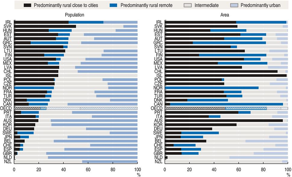
Note: The distinction between regions that are predominantly rural close to cities and those that are predominantly rural remote is not available for Australia, Chile, Korea, Latvia and Lithuania. For these countries “predominantly rural close to cities” refers to all predominantly rural areas.
Source: OECD (2016), Regions at a Glance 2016, https://doi.org/10.1787/reg_glance-2016-en.
Among the OECD residents living in predominantly rural regions, more than 80% live in rural regions close to cities representing one-fifth of the OECD population (21.4%). The remaining rural population living in remote rural regions amounts to 4.8% of the total share. However, the average hides significant differences across countries. In three countries (Slovak Republic, Ireland and Lithuania) the share of the population living in rural regions close to cities is at least 40% (Figure 3.4). While rural remote regions, despite their low aggregate share, account for more than one-quarter of the total population in three countries (Norway 32%, Greece 30% and Ireland 28%).
What are low-density economies?
Improving the categorisations of rural regions is vital for a better understanding of how rural economies perform and thus how to increase their productivity levels. Productivity growth in rural regions of the OECD countries is highly variable. As shown in Chapter 1, some have performed exceedingly well and are among the top 50 OECD regions in term of productivity growth. However, the majority of rural regions are not among the best performing regions in their country, which suggests the need for more analysis to determine what seems to drive productivity in rural economies. Before moving to this step, it is important to better describe how rural economies differ from urban economies. In this, it is useful to explore the idea of the “low-density economy” as a way to better understand what factors are important for economic growth. The low-density economy underpins an alternative model of economic growth that can be used to understand how rural regions can be high performing.
Low-density economies have specific characteristics related to proximity, density and location
Rural regions are fundamentally different than urban regions. Obviously they are smaller, less densely populated places with considerable distances between settlements, and consequently have different dynamics than urban areas. Unlike in cities where the “built environment” shapes most human behaviour, in rural areas it is the natural environment that mainly shapes human activities. While each rural place is unique it is still useful to generalise. For example, rural areas that are close to cities, which is the case for the vast majority in OECD countries, have different characteristics than those that are both rural and remote.
Rural regions that are well connected to cities will be linked to urban markets, whereas for remote rural areas, economic success is tied even more to the tradable sector. The tradable sector of the economy is that which concerns goods and services that are not restricted to local markets. The nature of these low-density economies, including their relative proximity to markets, socioeconomic dynamics, sectoral composition and so on, leads to very different types of places. As a result, they require different kinds of support to make the most of their assets and opportunities. These differences become more apparent at a more granular level of analysis (TL3 versus TL2 regions).
It is for these reasons that questions of economic geography loom large in the analysis of economic development in rural places. The geography of a place is effectively defined by a combination of physical (“first-nature”) and human (“second-nature”) geographies (Ottaviano and Thisse, 2004). The more people inhabit a place, the more its character will be defined by second-nature geography – by human beings and their activities. Where settlement is sparse, first-nature geography inevitably dominates – less human settlement and activity necessarily implies a larger role for natural factors, such as the climate or landforms, in shaping economic opportunities.
Peripherality in all its connotations can help us understand rural economies
Economic remoteness, or peripherality, which is always a relative term – is about being connected or unconnected to somewhere. Peripherality has three distinct dimensions. The first is simple physical distance to major markets. This increases travel times and shipping costs, which must be borne by the buyer (in the form of higher prices) or seller (in the form of lower margins). Yet straight-line distance is not all that matters: maritime transport is far cheaper and more flexible than overland transport, and it requires less dedicated infrastructure. Consequently, access to the sea is a crucial variable – southern Chile and coastal People’s Republic of China are far less remote from North American and European markets than, for example, Brazil’s Amazonian regions or China’s interior, respectively, even though these are physically closer to the main markets. Where overland distances are concerned, the quality and layout of infrastructure is clearly critical.
The second dimension of peripherality is the degree of economic connectedness. Lack of economic integration not only reduces current trade opportunities, it reduces the ability of agents in a place to identify new opportunities. Thus, there are costs in both static and dynamic perspectives. For example, Australian wheat farmers, though located in a very remote place, are extremely well connected, because they are deeply integrated into international grain markets and very well informed about changing conditions. By contrast, the residents of many small towns along the US Appalachian Mountains, which are among America’s poorest places, are physically very close to some of the world’s biggest factories and consumer markets, but they are poorly linked to those markets and thus largely disconnected from activities taking place only a short distance away.
The nature of low-density economies can be summarised in three dimensions (Figure 3.5). The first captures physical distance and the costs it imposes in terms of transport and more general connectivity of people. The second dimension is the importance of competitiveness in regions where the home market is small, the economy is highly specialised in the production of commodities, and all transport costs are absorbed by local firms. The third dimension of the figure captures the importance of “first-nature geography”, how the specific natural endowment shapes local economic opportunities.

Low-density economies located far from major markets tend to face a number of common problems
The principal sources of growth tend to be driven by external demand given the lack of internal markets. Since they can only produce a limited range of the goods and services they need, such regions are, out of necessity, orientated towards exports of one sort or another, unless they benefit from on-going income transfers. Otherwise, they cannot afford to import the goods they need from other places.
Local markets tend to be thin, with weak competition. This feature constitutes both a form of protection from external competitors, as well as a constraint on firm growth. While low-density places often have lower prices for land, prices for other goods and services may be higher than elsewhere, owing to weak competition. This is particularly true for remote regions, where high transport costs and the potential for suppliers to exploit their market power may more than offset the benefit of low land cost and non-tradable prices (i.e. the combination of low density and long distance can be especially expensive). Partly for these reasons, firms in such places tend to be dominated by small and medium-sized enterprises (SMEs), which are often low performing.
The economic structures of such places often have specific features. Production is concentrated in relatively few sectors, since it is impossible to achieve “critical mass” in more than a few activities. Whatever the respective roles of the primary, secondary and tertiary sectors, a narrower economic base implies greater vulnerability to sector-specific shocks, whether positive or negative. In a very large, dense economy, the greater range of activities typically offers a greater degree of resilience.
Most manufacturing in low-density economies tends to be “mature” in product-cycle terms. Although cutting-edge manufacturing tends to initially be concentrated in large cities, there are a wide range of examples verifying that they can also occur in rural regions (OECD 2014b). When they initially occur in large cities they can shift to more rural places later in the product cycle when at least one of two conditions holds: i) when proximity to some primary resource is important (e.g. the structure of transport costs is such that it is better to produce close to the resource rather than to the consumer market); and/or ii) where the technology is mature enough that the producers’ main concern is cutting production costs. In short, production often shifts to more distant places when the business is no longer rapidly growing. Where the latter motivation prevails, the tendency is to favour rural areas with good connections to major markets but low labour and real estate costs.
In rural settlements, volunteers often provide services that governments or firms provide in cities. The small populations of rural settlements often may make it unprofitable for a typical private firm to provide local services. In many rural places, residents band together to create a social enterprise that takes its place. For example, in England volunteers have kept open the local shop or pub when the previous owner realised profits were too low and chose to exit. Similarly, in North America small communities typically rely on volunteer fire departments because local governments cannot afford to staff a regular fire department. Without a strong group of volunteers, rural places would have much fewer local services and less access to goods, which would make them less desirable places to live (Osbourne, 2013). Moreover, volunteer organisations are also important pillars of social capital and can act as catalysts for economic and social initiatives (Schulz and Baumgartner, 2013).
Demographic change and low levels of educational attainment exert particular pressure on many low-density economies
OECD countries are ageing, and while this demographic pressure affects all regions, it does so more in rural regions and their low-density economies. This is especially challenging if the region is “peripheral”, i.e. located far from a city. The elderly dependency ratio, i.e. the ratio between the elderly population and the labour force, has been increasing for all types of regions over the last decade (Figure 3.6). While in most OECD countries, predominantly rural regions have a higher elderly dependency ratio than predominantly urban regions, those that are less peripheral, i.e. close to cities, have an elderly dependency ratio similar to that of urban and intermediate regions taken together.
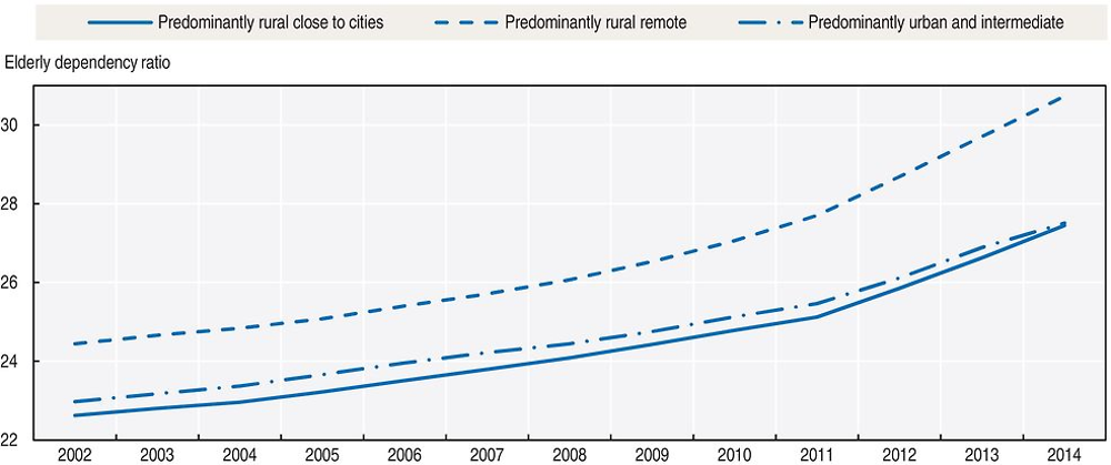
Source: Calculations based on OECD (2015a), OECD Regional Statistics (database), https://doi.org/10.1787/region-data-en (accessed 18 June 2016).
Rural regions also have an older population base than urban regions in all but seven OECD countries (Figure 3.7). In France and Portugal, the average age difference between the two types of regions is around five years. Conversely, in Poland, Estonia and Belgium, the average age in urban regions is about two years higher than in rural regions. There are also a number of countries for which the difference between the average age of the rural and the urban regions is rather small, such as Ireland, the Slovak Republic and Switzerland.
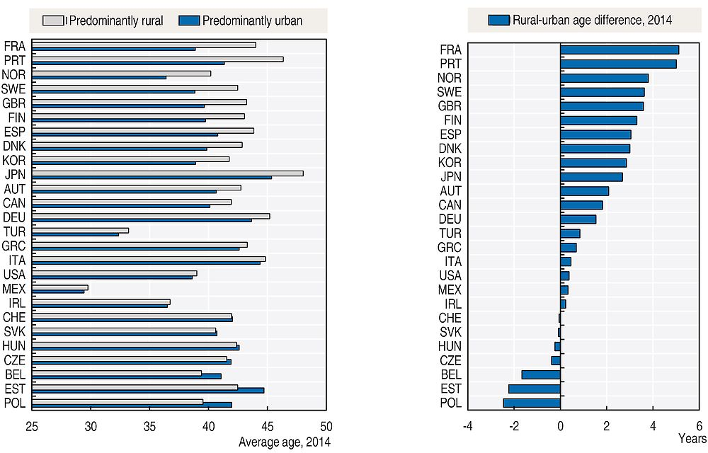
Note: Data for Mexico refers to 2010, all other countries data refers to 2014. Excluded OECD countries have missing values in at least one type of region.
Source: Calculations based on OECD (2015a), OECD Regional Statistics (database), https://doi.org/10.1787/region-data-en (accessed 18 June 2016).
The low-density economies in remote rural regions face mounting dual demographic pressures. Not only is the elderly dependency ratio higher than in other regions and the gap between rural remote regions and other types of regions has widened over time, but the youth dependency ratio – defined as the share of the population under 15 years, over the working age population – is higher in rural regions compared to urban and intermediate regions. This means that rural regions tend to have a larger share of their population that is not in the labour force, either because they are too young or too old, but who require access to education, health and other public services.4 These population dynamics can lead to a shrinking local labour market and present a potential fiscal problem for the regions that need to rely more on transfers than local taxes. Moreover, providing services for the elderly and young can place pressure on a small labour force and reduce average productivity because the services provided tend to have a low level of worker productivity, especially where economies of scale cannot be achieved. In rural areas close to cities, policies can try to address these population dynamics by enhancing rural-urban linkages, which facilitate the access to services mainly located in urban areas (such as specialised health care for the elderly and educational opportunities for young people).
Low levels of educational attainment in rural areas limit opportunities for productivity growth in their low-density economies
Human capital and skills are critical drivers of regional growth, and this is particularly challenging for rural regions that may suffer from “brain drain” (OECD, 2012). The labour market for high-skilled workers tends to be global and dominated by cities and large metropolitan areas, given the opportunities and amenities they offer through the presence of economies of agglomeration. In contrast, the market for low and technical skills is much more locally driven. This suggests that the productivity of rural areas depends on the successful upgrading of low-skill workers and an increase of workers with technical skills. Research finds strong benefits of reducing the share of low-skilled workers in the regional labour force supports economic growth (OECD, 2013). This result is particularly relevant for rural regions, where policy should focus on retaining youth in schools, matching the supply of skills to available jobs in the labour market and to prioritise technical skills, rather than scientific skills.5
Low levels of high-skilled workers can be a bottleneck for growth in low-density economies. Educational attainment provides an indicator for the average skill level in the labour force. The share of workers with tertiary education, i.e. a university degree, is lower in regions characterised by low-density economies, while the share of workers that do not have education beyond primary education (a proxy for low-skilled workers) tends to be high in these regions. Put differently, rural regions tend to have a higher share of low-skilled workers.
The skills gaps between urban and rural regions can be substantial. The percentage of university educated workers in the most rural (TL2) regions is lower than in the most urban regions in each OECD country with available data. For example, in Denmark and Sweden the share of workers with tertiary education in the most urbanised regions is 50% higher than in rural regions (Figure 3.8). The difference in terms of the workforce with only primary education is significantly smaller in Sweden (15% higher in rural compared to urban areas) than in Denmark (36%). This is in contrast to Hungary and Greece, where rural economies have both significantly lower shares of workers with tertiary education and significantly higher shares of workers that did not progress beyond primary education. In two countries, Germany and the United States, the share of only primary educated workers is higher in urban regions. In Germany, this partly reflects the historic east-west divide and the significantly lower shares of workers with only primary education in the (less densely populated) east of Germany. It also reflects that there are three Länder that are (administrative) cities and that cities often have a workforce with many workers at both ends of the skill spectrum. For the United States the difference is driven by states that are mostly urbanised and have a large percentage of foreign born residents (see Chapter 1 for a discussion of inclusion and migration in cities).
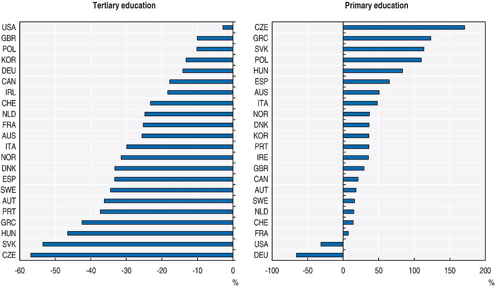
Note: Each bar represents the percentage difference between the share of the labour force with tertiary (primary) education in regions in a country that belong to the 25% of OECD TL2 regions with the lowest share of population in low-density economies (the most urban regions) compared to those among the 25% with the highest share of population in low-density economies (i.e. the most rural regions).
Source: Calculations based on OECD (2015a), OECD Regional Statistics (database), https://doi.org/10.1787/region-data-en (accessed 18 June 2016).
Productivity and innovation are directly linked to the characteristics of low-density economies
Low-density economies are, almost by nature, characterised by limited diversification of economic activity. Smaller places with small labour forces cannot achieve critical mass nor economies of scale in very many activities. This also means that local producers often face thinner markets for their inputs – a lack of redundancy in markets can mean that weakness in one part of a supply chain harms other firms in the chain. It is not so easy to replace a supplier who fails or is underperforming in terms of quality or price. Low levels of diversification thus imply heightened vulnerability to external shocks, particularly those affecting the “export base” sectors.
As a consequence of many of these factors, such places tend to have lower levels of productivity, except in the primary sector, and limited entrepreneurial activity. Entry rates for new firms are typically lower than in denser places. Other things being equal, cities offer new firms a richer “ecosystem” in which to develop. In addition, the opportunity costs of failure in big, dense economies tend to be lower (resources released in the event of a failure are easier to reallocate to other uses) and, in part for that reason, the cost of capital tends to be lower as well.6 Survival rates for new firms, though, are often higher in less dense economies, because entrants have to be fairly productive in order to overcome the barriers to entry (OECD, 2011b).
In general, levels of patenting and formal research and development also tend to be low, though low-density economies can be surprisingly innovative in ways that traditional innovation indicators do not capture. In more remote rural regions, the incentives to innovate may be high. It can be difficult to purchase an existing solution to a problem for an individual or firm. This reflects the narrow range of existing local suppliers and difficulties in identifying distant potential suppliers. Further, distance creates barriers to competition that can enable entrepreneurs to “capture” or monopolise local markets. However, unless these entrepreneurs are low-cost producers or have unique products, it will be difficult for them to expand beyond the local market.
Place matters because places are different. Territorial policies take this seemingly simple statement as a starting point and use it to construct initiatives and interventions to support the development of cities, regions and communities in an inclusive, robust and sustainable manner. Different places have their own unique assets and attributes and, as a result, it is important to understand different geographies, contexts and institutions, in order to adopt the most effective policies and support local actors. This is particularly important for rural places because of their extremely diverse characteristics and the structure of low-density economies. The next section explores the differential trends in different types of rural areas in more detail.
Trends, opportunities and challenges for rural areas
Rural areas often have substantial growth potential. This has been highlighted in previous empirical work on the determinants of regional growth and is reflected in the results presented in this section. It is important to note that the productivity performance of rural regions has implications for national performance. National levels of productivity are built up from regional levels, which in turn reflect the productivity of individual firms. While the level of economic activity in individual rural regions is small, the aggregate contribution of rural regions to national growth is significant because there are many of them. Moreover, the viability of firms in rural regions may hinge on them having relatively high productivity, because they must compensate for higher transport costs than urban peers. Consequently rural firms may even make a disproportionate contribution to national productivity that goes beyond their number.
Rural regions have, on average, performed relatively well in terms of productivity growth, but were harmed by the recession. Chapter 1 shows that the gap in productivity growth has been increasing across all OECD regions, but this divide is not between urban and rural regions, but rather between a small number of urban and rural regions and all other regions (rural and urban included). However, on average, rural regions have lower levels of GDP per capita and lower levels of productivity than urban regions, with levels in both measures below the national average in their respective countries. However, the best performing regions in terms of growth are a mix of predominantly urban and predominantly rural regions. This suggests that mechanisms for productivity growth are available to rural regions and not only to those that are urban.
In terms of growth rates over the period 2000-07, rural regions performed very well. They recorded an average annual rate of growth (GDP per capita) of around 2.3%, which is close to the average growth rates of urban regions (2.4%) and above the intermediate regions (2.2%). Yet, while rural regions performed well before the global financial crisis, they were the most vulnerable regions since the onset of the crisis, with an average drop in GDP per capita of -1.11% annually over the period 2008-12. This variability in performance suggests that rural economies face particular challenges inherent in low-density economies (as discussed above). In particular the limited diversification of economic activity, problems with accessibility, lack of critical mass and population ageing, accentuated by the outmigration of young people limit their resilience.
Trends in regional productivity
Rural regions are not synonymous with decline
The widespread perception that “rural” is somehow synonymous with “decline” in OECD countries is simply wrong. In the run-up to the financial and economic crisis (2000-07), all rural regions combined recorded an average annual growth rate of just under 2% in labour productivity (real GDP per worker) and 0.12% since the crisis (2008-12) (Table 3.2). This is higher than the average growth rates of urban and intermediate regions, which, before the crisis, grew at 1.7% and 1.6% respectively. The contraction of productivity growth since the crisis was however larger in rural regions than in the other two categories. This is also reflected in the relative position of regions across OECD countries. Urban and intermediate regions improved their performance compared to the OECD average in GDP per capita from 2000 to 2012, while rural regions fell further behind (Table 3.2, upper panel). However, this does not reflect the reality for the majority of the rural population. Rural regions close to cities narrowed their gap to the OECD average GDP per capita levels by more than urban and intermediate regions pulled away. Remote rural regions account for most of the increased gap among all rural regions.
Rural regions close to cities perform particularly well
The downturn since the crisis has affected remote rural regions much more than rural regions that are close to cities. When rural is divided into two constituent parts, the two types of rural regions perform very differently. The regions that are “predominantly rural close to cities” display higher productivity growth before the crisis and more resilience after the crisis began. The economies of predominantly rural remote regions show a very different pattern. They are the most badly affected by the crisis, with an annual average drop of GDP per capita of -2.5%, more than 2 percentage points worse than rural regions close to cities. Productivity declined as well in the period 2008-12, albeit at a slower pace with an annual average decline of -0.6%. While slower, the decline is still a full percentage point more than in rural regions close to cities. This shows that the weaker performance of rural regions in aggregate mainly reflects rural remote regions, where productivity contracted.
The attractiveness of rural areas that are close to cities is also reflected in population growth figures. Predominantly urban regions and intermediate regions experienced stronger population growth than rural regions combined. But this is driven by remote rural regions declining, on average, between 2000 and 2007 and growing by less than 0.2% per year between 2008 and 2012. The population in rural regions close to cities grew by about 0.6% during those periods. This is a low growth rate, but only slightly lower than the rate in urban regions and higher than for intermediate regions.
Performance varies more across rural regions than it does in intermediate and urban regions
The average performance of regions masks a high degree of variability. The standard deviation of labour productivity growth captures the range of growth rates across TL3 regions. It is higher for rural regions than for urban or intermediate regions (Table 3.3). In particular remote rural regions show very high variability, as exhibited by their high coefficient of variation (the ratio of standard deviation and the average growth rate). This variability reflects the fact that rural regions have a tendency to either do well or poorly, i.e. rural performance tends to cluster at the extremes as they exhibit boom and bust economies.
This variation is further accentuated when growth across the whole distribution of urban and rural regions is considered (Figure 3.9). A higher estimated density indicates that a higher share of regions fall around the specified growth rate. Across all types of regions the annual average growth rates are less-widely spread over the whole period analysed (2000-12) than before or since the crisis. In all three periods, rural regions close to cities outperform rural remote regions in all parts of the distribution, which is indicated by the distribution being further to the right (Figure 3.9, upper row). This means that, for example, regions in the bottom 20% of rural regions close to cities grew faster than the bottom 20% of regions that are rural remote. The difference is even more pronounced compared to predominantly urban regions. Urban regions have a higher peak, indicating stronger clustering of regions around average growth rates, than remote rural regions. This is combined with a narrower distribution for urban regions, which means that there are fewer regions with extreme growth events. The left tail, indicating low growth or decline, in particular is much less pronounced in urban regions than in remote rural regions. This pattern is in line with a lack of diversification in remote rural economies.

Note: Labour productivity is defined as GDP per employee. GDP is calculated at PPP constant 2010 USD, regional employment is measured at place of work.
Source: Calculations based on OECD (2015a), OECD Regional Statistics (database), https://doi.org/10.1787/region-data-en (accessed 18 June 2016).
Linkages between rural and urban areas are key mechanisms for diffusing productivity
Urban regions tend to have higher levels of productivity. Table 3.2 shows that in 2012, average productivity in urban regions measured by GDP per capita was 21% above the OECD average for TL3 regions. Some of the factors driving this higher level of urban productivity may benefit adjacent rural regions as well. For example, agglomeration effects can “spill” across a broader geographical area and reach rural regions, even when the connections between rural and urban regions are not particularly strong. This may be a factor explaining the relatively strong performance of rural regions close to cities. One of the main policy concerns of countries is how to foster productivity by favouring the diffusion of technology from the frontier. Proximity, reinforced by enhanced linkages between rural and urban areas, may well be such a diffusion mechanism.
The strong performance of rural regions close to cities is not solely linked to their proximity to a large metropolitan area. Indeed, the definition of “rural close to cities” refers to any city of more than 50 000 inhabitants. This highlights the role played by small and medium-sized cities for the economic development of rural regions, but benefits cannot be achieved without access. This highlights the importance of transport links for rural areas, especially given a low population density. At least half of a region’s population that is “close to a city” can access services provided by the city in less than 60 minutes driving distance, the population of “remote” rural areas needs to drive even further. But in both cases, “borrowing” the agglomeration benefits of large metropolitan areas, i.e. the largest cities across the OECD, might require bridging longer distances. Therefore, accessibility is a challenge for all rural areas, but seems to also play a key role in supporting the strong economic performance of rural regions close to cities.
Productivity trends among small (TL3) regions in the OECD
Rural regions are well represented in the top performing regions in terms of productivity growth, particularly rural regions close to cities
Rural regions accounted for half of the top 10% fastest growing OECD regions in terms of labour productivity before the crisis. Even after the onset of the crisis 40% of the fastest growing regions were rural. Before the crisis, rural remote regions and rural regions close to cities were leveraging their “catching up potential”. While they initially had relatively low labour productivity levels, they experienced significant productivity growth, in excess of 4% per year, before the crisis (Figure 3.10). Since the crisis, a significant share of rural regions remain among the fastest growing regions, but with a greater shift towards rural regions that are close to cities. Among the 10% fastest growing TL3 regions in the period before the crisis, half are rural regions, overrepresented are rural regions that are close to cities (36%). In the following period, the number of rural regions in the top performing group declined to 41%, with the largest decline occurring amongst rural remote regions, representing only 9% of top-performing regions.

Note: TL3 regions are selected according to their labour productivity growth rate before and since the crisis. Labour productivity is defined as real GDP per worker. GDP is calculated at PPP constant 2010 USD, regional employment is measured at place of work.
Source: Calculations based on OECD (2015a), OECD Regional Statistics (database), https://doi.org/10.1787/region-data-en (accessed 18 June 2016).
The resilience of rural regions close to cities may be the result of economies of “proximity”. As discussed above, a strong link between urban regions and adjacent rural regions may have been beneficial in times of economic expansion and also in times of decline, given the stronger resilience of urban regions to downturns due to their thicker markets and more diversified economic base. The evidence of the good productivity growth in rural regions close to cities highlights the importance of fostering rural-urban linkages in these regions, especially since the highest levels of labour productivity tend to be in urban areas. Remote rural regions were fewer than one in ten among the 10% OECD TL3 regions with the highest levels of labour productivity. Since the crisis, no remote rural region belongs to this group of highly productive regions. Conversely, urban regions represent 68% of the most productive regions, underlining the importance of agglomeration benefits.
Increasing productivity is a key strategy for rural regions, but the nature of such increases matters
Increasing productivity, i.e. output per worker, is perhaps the most important way to increase the competitiveness of firms and regions in order to boost worker wages, opportunities and well-being. However, a common mechanism to increase productivity is to substitute capital for labour in the production process. In this case, if output remains constant, there is an obvious need for a reduction in the number of workers, or in the hours worked per worker. Alternatively, a firm that faces declining sales may lay off workers, but this may result in higher output per worker for those who remain, either because employers selectively eliminate the least effective workers or because the fixed stock of firm capital is spread over a smaller employment base, which might result in higher output per worker. Both of these strategies have the obvious benefit of keeping the firm operating, but both lead to negative impacts on the part of the local labour force.
The ongoing modernisation process, whereby labour is substituted for capital, might lead to the so-called “rural paradox” resulting in job losses and regional decline. This refers to the fact that rural regions may boost productivity by “shedding” labour, i.e. by reducing employment. The “paradox”, when productivity growth is driven by a reduction of employment, is that productivity growth creates challenges for an inclusive and sustainable path of development, rather than support it. These challenges can be quite important for the mid- and long-term resilience of rural communities. If the laid-off workers leave the region, an already thin labour market is shrinking further, with serious consequences for the development prospects of the region. In this sense, the “rural paradox” could make rural regions become victims of their own success.
In most cases, higher productivity has been associated with increasing employment
The “rural paradox” is however not the rule. Increases in productivity can result in a larger output volume for the improving firm and region, either through increasing market shares, i.e. displacing competing low-productivity, high-cost firms, or from a general increase of industry demand, due to the reduction of prices or increases in the quality of the products. In these cases, higher productivity is associated with an increase in employment.
The analysis over the period 2000-12 reveals no evidence of a general “rural paradox”, but since the 2007-08 crisis, rural regions struggle to combine productivity and employment growth. The majority of TL3 regions, including both rural and urban ones, that had positive productivity growth in the pre-crisis period, also display positive growth of both GDP per capita and employment. In particular, 69% of rural regions that are close to cities and 64% of remote rural regions combined productivity and employment growth (Figure 3.11). A positive correlation between GDP per capita growth and employment growth is present both before and since the crisis. The main difference between the two periods is a shift of the whole distribution from a situation of mainly positive growth of GDP per capita and employment to a situation of mainly no growth, exhibited by a clustering of regions around the origin of Figure 3.11 (lower panel). Since the crisis, the number of rural regions experiencing both positive productivity and employment growth dropped to 36, i.e. to only 13% of rural regions, compared to 192 (67%) before the crisis.
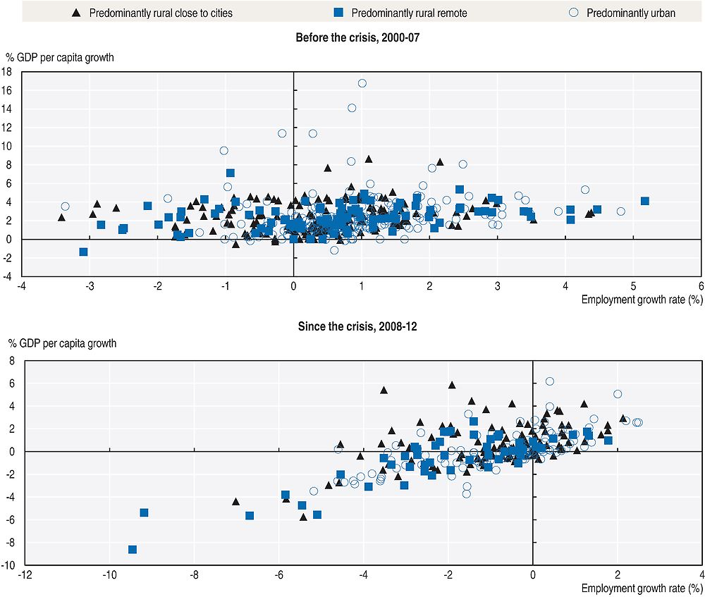
Note: Only the sub-sample of OECD TL3 regions with positive labour productivity growth are included in the graphs. GDP is measured at PPP constant 2010 USD, and regional employment is measured at place of work.
Source: Calculations based on OECD (2015a), OECD Regional Statistics (database), https://doi.org/10.1787/region-data-en (accessed 18 June 2016).
Among rural regions, the simultaneous increase of productivity and jobs is more frequent in rural regions close to cities
Among sub-types of rural regions, the majority of dynamic rural regions close to cities are becoming more productive and increasing employment simultaneously. But, the 2007-08 economic and financial crisis led to reductions in GDP and employment. The number of regions with increasing GDP per capita, but decreasing employment is larger than in the period before the crisis (Figure 3.12). Many remote rural regions in particular suffered doubly, both GDP per capita and employment declined following the global shock in 2007-08. Only 6% of rural remote regions displayed both productivity and employment growth since the crisis, compared to 16% of rural regions close to cities. These trends may be consistent with the importance of the tradable sector in rural regions which drove the virtuous cycle of increasing GDP and employment before the crisis and which was badly hit by the collapse of global trade in the years since the 2007-08 shock.
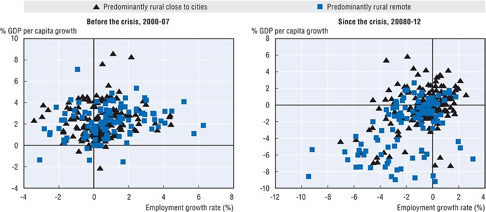
Note: OECD TL3 rural regions. GDP measured at PPP constant 2010 USD.
Source: Calculations based on OECD (2015a), OECD Regional Statistics (database), https://doi.org/10.1787/region-data-en (accessed 18 June 2016).
What are the key factors driving these trends?
The accumulation of capital (physical and human) and the pace of innovation are key
In a globalised economy, firms and regions are required to compete internationally, and their competitiveness is strongly linked to productivity. Regional performance is driven by a combination of interconnected factors that include: geography, demography, specialisation, institutions, physical and human capital, and the capacity to innovate (OECD, 2009; see also Chapter 1). Some factors refer to the national regulatory and macroeconomic scenario that may favour the competitiveness of some regions within a country. Others, however, refer to specific regional characteristics. Among them, the most important refer to the accumulation of capital, both physical and human, and the pace of innovation.
The following analysis looks at characteristics that distinguish successful rural regions. Based on available data, it is possible to consider several characteristics of the regional economy, the labour market (employment rate, unemployment rate, and participation rate), demography (population density and elderly dependency ratio), and sectoral specialisation (manufacturing and the tradable sector). In order to include the largest possible number of regions in the analysis, the period before the crisis is limited to the period 2004-07. Both before and since the crisis, successful regions are here defined according to their labour productivity growth rate. The group of successful regions refers to the top 40% of regions in terms of labour productivity growth and the group of unsuccessful regions refers to the bottom 40% of the distribution.
Tradable activities are key drivers for rural productivity growth
What stands out among the characteristics of successful and unsuccessful rural regions is the importance of the tradable sector (Table 3.4 and Figure 3.13). Before the crisis, the contribution to total output produced by the manufacturing sector was 24% in successful rural regions close to cities and 20% in remote rural regions. This is a substantial difference to the 16% and 11% contribution of manufacturing in the least successful rural regions. This difference reinforces the results from Chapter 1 that highlight the role of the tradable sector for productivity growth. For rural regions, manufacturing is a major part of this result. But, other tradable sectors also contribute, as is evident in the difference for rural regions close to cities, where 40% of output in successful regions is produced in the tradable sector as opposed to 29% in the least successful regions. This confirms the importance of tradable activities for the overall performance of rural regions, given their lack of a large internal market and lower productivity of the services sector due to lack of agglomeration economies. It suggests that the common emphasis of rural policy on stimulating manufacturing and other tradable sectors has considerable merit.
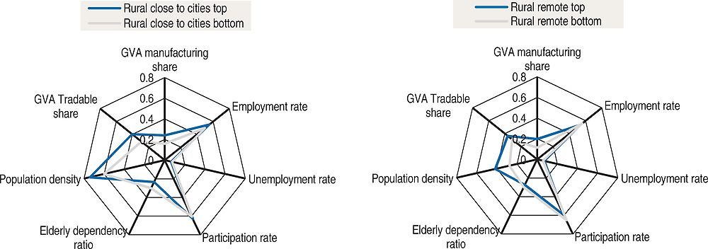
Note: All indicators represent shares; the scale goes from 0 to 1, except for population density, which is measured as 100 residents per km2.Top refers to rural regions in the top 40% of growth of GDP per worker in the relevant period. GDP and GVA are measured at PPP constant 2010 USD, SNE2008 classification; employment is measured at place of work. The tradable sectors are: agriculture (A), industry (BCDE), information and communication (J), financial and insurance activities (K), and other services (R to U). The manufacturing sector is a subset of the tradable sector.
Source: Calculations based on OECD (2015a), OECD Regional Statistics (database), https://doi.org/10.1787/region-data-en (accessed 18 June 2016).
The large difference in the contribution of tradables is contrasted by small differences in labour market-related characteristics, with some indication of demographic challenges curtailing growth. The difference in employment, unemployment and participation rates between the top 40% and the bottom 40% of regions in both rural regions close to cities and remote rural regions is small, with little discernible pattern (Table 3.4 and Figure 3.13).7 The elderly dependency ratio, i.e. the total population above the age of 65 compared to the labour force is higher in less successful regions, indicating a potential bottleneck for rural growth. Population density (especially in rural remote regions) is another element of distinction of successful regions. The importance of population density for the economic performance of rural regions suggests that a “minimum” level of density is crucial in order to take advantage of economies of scale and scope for the delivery of goods and services. This is another factor that helps explain why rural regions close to cities tend to outperform rural remote regions. Along with the promotion of the tradable sectors, public policy in rural remote regions should also facilitate connections between isolated communities.
Rural remote regions have suffered more since the financial crisis than rural regions close to cities
The analysis of the period 2008-12 provides some indication of the resilience of rural economies to the global crisis. Sector specialisation seems not to matter for rural regions close to cities. The groups of top and bottom performing regions have both similar shares of gross value added (GVA) in tradable sectors and GVA in manufacturing, 36% and 22%, respectively (Table 3.5 and Figure 3.14). This lack of difference may reflect the drop in international trade and global demand which reduced the importance of the tradable sectors for growth. This suggests that specialisation in the tradable sectors can boost productivity, but that rural regions remain vulnerable to global crises that affect international trade flows, such as the global shock of 2007-08 and the subsequent period of recession.
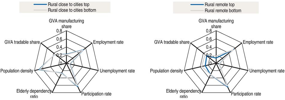
Note: All indicators represent shares; the scale goes from 0 to 1, except for population density, which is measured as 100 residents per km2. Top refers to rural regions in the top 40% of growth of GDP per worker in the relevant period. GDP and GVA are measured at PPP constant 2010 USD, SNE2008 classification; employment is measured at place of work. The tradable sectors are: agriculture (A), industry (BCDE), information and communication (J), financial and insurance activities (K), and other services (R to U). The manufacturing sector is a subset of the tradable sector.
Source: Calculations based on OECD (2015a), OECD Regional Statistics (database), https://doi.org/10.1787/region-data-en (accessed 18 June 2016).
Rural remote regions present a different picture, as the most resilient regions are those where the share of GVA from the tradable sector is lower. The results for population density suggest a regional switch in performance, with the most dynamic regions before the crisis losing heavily since the global shock in 2007-08, with the initially poorer performers before the crisis displaying a better resilience since the crisis. Whether this performance is sustainable is another question, as this better performance of the most remote regions, with lower population density, and a lower share of the economy based on tradable sectors, probably reflects a regional economy based on the public sector and financed through transfers from the central government, which are (by nature) less dependent on the business cycle and less responsive to macroeconomic shocks – at least in the short term.
Conclusion
The chapter extends the idea from Chapter 1 that productivity growth can occur in any type of region and focuses on the rural regions of the OECD. To understand rural growth dynamics it is important to first understand how rural regions differ, because differences in conditions affect the potential for growth. To this end, the chapter introduces the idea of a “low-density economy” that highlights the importance small home markets, physical distance and the role of the local environment for rural areas. The OECD is now employing a typology of regions that uses the degree of physical distance from, and the degree of connectivity to, an urban centre as way to categorise three degrees of rurality. Development opportunities and constraints vary considerably among the three categories and these can lead to differences in relative performance.
The empirical evidence highlights the significant growth potential of rural regions, but it also shows that significant differences in performance exist among different types of rural regions. In terms of productivity growth, rural regions close to cities outperformed urban regions, both before and since the crisis. In contrast, the performance of rural remote regions was significantly weaker, underlining the importance of spillover effects between urban regions and adjacent rural regions and the need to better understand rural-urban linkages. This is particularly important when it comes to economic resilience of rural economies, as the main distinguishing feature between successful and unsuccessful rural regions since the 2007-08 crisis seems to be their proximity to urban centres.
Tradable activities appear to be a crucial factor driving the performance of rural regions, as was shown to be the case for all types of regions in Chapter 1. The presence of tradable activities (e.g. agriculture, manufacturing, energy, mining, and financial and business services) represents the main discriminant between the strong and poor performers before the crisis period. For both rural regions that are close to cities and remote rural regions, the strong performers systematically have a higher share of GVA in tradable activities than the underperformers. In addition, amongst remote rural regions, strong performers have higher population density which suggests that reaching a certain degree of density is a critical driver of performance for low-density economies. Boosting productivity in rural regions can also be inclusive and sustainable, as the majority of dynamic rural regions are boosting their productivity while creating jobs.
Rural growth can take place and some rural regions are high performing in terms of productivity growth rates, however, most rural regions do not perform well. In many cases they lack some of the prerequisites for growth outlined above. A role for public policy for rural regions is to help support the establishment of these prerequisites. Chapter 4 takes on the challenge of identifying a rural policy framework – Rural Policy 3.0 – that builds on the ideas of the New Rural Paradigm (OECD, 2006) as a way to increase the economic performance of rural regions so they can make a full contribution to national growth and reduce current levels of spatial inequality.
Bibliography
Brezzi, M., L. Dijkstra and V. Ruiz (2011), “OECD Extended Regional Typology: The Economic Performance of Remote Rural Regions”, OECD Regional Development Working Papers, No. 2011/06, OECD Publishing, Paris, https://doi.org/10.1787/5kg6z83tw7f4-en.
Eurostat (n.d.), Urban Rural Typology, http://ec.europa.eu/eurostat/statistics-explained/index.php/Urban-rural_typology (accessed 20 June, 2016).
INSEE (L’Institut national de la statistique et des études économiques) (2016), “L’accessibilité aux services de la vie courante : un temps d’accès lié à la densité de population”, www.insee.fr/fr/themes/document.asp?reg_id=29&ref_id=23861 (accessed 20 June 2016).
OECD (2016), Regions at a Glance 2016, OECD Publishing, Paris, https://doi.org/10.1787/reg_glance-2016-en.
OECD (2015a), OECD Regional Statistics (database), https://doi.org/10.1787/region-data-en (accessed 18 June 2016).
OECD (2015b), “OECD Regional Outlook Survey”, GOV/RDPC(2015)8, OECD, Paris.
OECD (2014a), OECD Rural Policy Reviews: Chile 2014, OECD Publishing, Paris, https://doi.org/10.1787/9789264222892-en.
OECD (2014b), Innovation and Modernising the Rural Economy, OECD Publishing, Paris, https://doi.org/10.1787/9789264205390-en.
OECD (2013), Rural-Urban Partnerships: An Integrated Approach to Economic Development, OECD Publishing, Paris, https://doi.org/10.1787/9789264204812-en.
OECD (2012), Promoting Growth in All Regions, OECD Publishing, Paris, https://doi.org/10.1787/9789264174634-en.
OECD (2011a), OECD Regional typology, https://www.oecd.org/gov/regional-policy/OECD_regional_ typology_Nov2012.pdf.
OECD (2011b), OECD Regional Outlook 2011: Building Resilient Regions for Stronger Economies, OECD Publishing, Paris, https://doi.org/10.1787/9789264120983-en.
OECD (2009), How Regions Grow: Trends and Analysis, OECD Publishing, Paris, https://doi.org/10.1787/9789264039469-en.
OECD (2006), The New Rural Paradigm: Policies and Governance, OECD Publishing, Paris, https://doi.org/10.1787/9789264023918-en.
Osborne, S.P. (2013), Voluntary organizations and innovation in public services, London: Routledge.
Ottaviano, G. and J.F. Thisse (2004), “Agglomeration and economic geography”, Handbook of Regional and Urban Economics, Vol. 4, pp.2563-2608.
Schulz, T. and D., Baumgartner (2013), “Volunteer organizations: odds or obstacle for small business formation in rural areas? Evidence from Swiss municipalities”, Regional Studies, Vol. 47(4), pp.597-612.
Statistics New Zealand (2016), Defining Urban and Rural New Zealand, www.stats.govt.nz/browse_for_stats/Maps_and_geography/Geographic-areas/urban-rural-profile/defining-urban-rural-nz.aspx (accessed 20 June, 2016).
The test of mean difference allows the statistical reliability of the observed differences in the mean values of different types of regions to be established.
In 2015, the OECD Regional Database was updated according to the 2008 revision of the System of National Accounts (SNA 2008) and, for the real value indicators, a new base year (2010) is considered. Regional indicators are in the process of being updated so that the new series covers a smaller number of OECD countries than the old series. The text uses the new system of accounts (SNA 2008) although it covers a smaller sample of regions, because it provides better international comparison and easier verifiability, as data for the prior revision (SNA 1993) are no longer publicly available.
Nevertheless, in order to lend support and verify the robustness of the results based on the SNA 2008, the same statistics are computed with the 1993 SNA definition, using the larger number of regions available under the previous revision. The main difference between the two series is the absence of regions from Japan, Korea, Italy and Norway in the new series. This is due to a time lag in the updating process and statistics will become available soon. Table 3.A2.1 shows that although the coverage in terms of total number of regions is different (788 compared to 868) the distribution of regions across the regional typologies is quite similar. The comparison also shows that the key results discussed in this chapter are also present in the SNA 1993 data (Table 3.A2.2).
Notes
← 1. The statistical data for Israel are supplied by and under the responsibility of the relevant Israeli authorities. The use of such data by the OECD is without prejudice to the status of the Golan Heights, East Jerusalem and Israeli settlements in the West Bank under the terms of international law.
← 2. The EU’s urban-rural typology uses a three-step approach to classify the NUTS level 3 regions. Rural areas are defined by: identifying populations in all areas outside urban clusters; classifying NUTS3 regions on the basis of the share of their population in rural areas; and differentiating between predominantly rural and intermediate regions. See: Eurostat (n.d.), Urban Rural Typology, http://ec.europa.eu/eurostat/statistics-explained/index.php/Urban-rural_typology (accessed 20 June 2016).
← 3. The method differs from the OECD approach in three key ways: i) it considers not only population density but also the share of agricultural area as a discriminatory variable; ii) the classification is at the administrative unit (municipality or communal level), while the OECD method uses the small region (TL3) level (in this case provinces) with several problems of inner heterogeneity; and iii) the classification is performed within each geographical area (mountain, hill and plain), with the purpose of taking into account different natural and soil endowments.
← 4. A consequence of this is that estimates of productivity expressed on a per capita basis tend to depict rural regions less favourably than estimates based on a per worker basis.
← 5. The effects of human capital on productivity can only be assessed for TL2 regions, because of data limitations – indicators of human capital are not available at a lower regional level (e.g. the TL3 level used throughout this chapter). The OECD typology, which classifies regions in predominantly urban, intermediate, and predominantly rural, is not available at the TL2 level. To overcome this problem and to make inference between educational outcomes and rural characteristics, the present analysis uses an index of rurality which captures the share of regional population living in rural areas. It defines four categories of TL2 regions ranked by regions with the highest share of population living in rural communities to regions with the lowest.
← 6. Lenders must always consider the potential value of collateral: in a denser economy, it is likely to be higher because deeper markets imply greater opportunities for reallocation of assets. To take a simple example, if a borrower builds a plant in a large city and then goes out of business, the building and grounds are likely to be easier to resell advantageously than if he builds the same plant in a small town, where it may stand empty and derelict for a long period.
← 7. The descriptive analysis illustrates differences in average characteristics of fast- and slow-growing rural regions that can be indicative of determinants or drivers of labour productivity. Establishing a causal link between the characteristics and growth requires more in-depth analysis.