Chapter 3. Sprawl in OECD urban areas
This chapter operationalises the conceptual definition of urban sprawl offered in Chapter 2 and provides a cross-city and cross-country analysis of the phenomenon. The different dimensions of sprawl are represented by indicators that are computed using three data sources: two high-resolution global datasets on land cover and population, and the geographic delimitation of functional urban areas. The indicators are computed for 1 156 urban areas in 29 OECD countries. They are then used in cross-city and cross-country comparisons, as well as in a country-level analysis of urban sprawl. The findings show that many cities and countries have been sprawling since 1990, even though this process is manifested in heterogeneous ways. Among the dimensions of urban sprawl, fragmentation of urban land, variation of urban population density and the share of urban land allocated to very low density levels have grown in most countries since 1990. At the same time, urban areas in some countries, including Austria, Canada, Slovenia and the United States, rank high in multiple dimensions of sprawl, while cities in other countries, such as Czech Republic, Denmark, France, Hungary, Poland and Slovak Republic have been sprawling along most of the considered dimensions since 1990.
3.1. Introduction
Urban sprawl is a concept that can be operationalised and measured exclusively within city limits; therefore, well-defined delimitations of urban areas are a prerequisite for the effective study of the phenomenon. This chapter provides an inter-temporal, cross-country analysis of sprawl in OECD urban areas. The analysis is based on the measurement of urban sprawl that has been conceptualised in Chapter 2. That is, each indicator proposed in this chapter corresponds to an urban sprawl dimension discussed in that chapter. In contrast to several complex sprawl indicators analysed in earlier studies, the metrics1 proposed here can be more directly related to the effects of certain policies, such as the ones discussed in Chapter 4. The urban form indicators are measured for 1 156 urban areas in 29 OECD countries. Data from three different sources are combined to compute them: i) a unique dataset that identifies built-up areas globally with a resolution of 38 m × 38 m at three different time points (1990, 2000 and 2014); ii) a dataset on global population density with a 250 m × 250 m resolution observed for the same time points; and iii) a geospatial dataset designating the borders of OECD urban areas.
The outline of the chapter is as follows. 3.2 provides a systematic review and classification of metrics used to operationalise the multiple and diverse definitions of urban sprawl in the literature. 3.3 describes the three main data sources used in the current study, where special attention is paid to the dataset on geographic delimitation of urban areas. 3.4 briefly describes the urban sprawl indicators used in the study, and visualises and discusses the most important findings from a cross-country analysis of these indicators. 3.5 presents some results of the country-level analysis, which is further elaborated in Appendix 3.B. 3.6 concludes.
3.2. Background literature
Urban sprawl has been analysed by various disciplines such as landscape ecology, transport planning, geography and urban economics, each with their own point of view on the concept (Arribas-Bel, Nijkamp and Scholten, 2011). There is no consensus on the definition of sprawl and the way to quantify it. However, it is widely accepted that urban sprawl is a multidimensional concept whose definition on the basis of average population density or occupied urban footprint may be too simplistic. As highlighted in Chapter 2, the distribution of population may vary widely across urban areas with identical average population density, even if the areas occupy the same footprint. Therefore, the entire distribution of population across space is central in comparing urban areas. Compact development around major public transport nodes can provide an average density that is equally low to that of a suburban zone where development is scattered. However, the environmental, economic and energy profiles of the two suburban areas may be diametrically opposed. Therefore, several dimensions are required to describe urban sprawl in a meaningful way (see e.g. Galster et al., 2001; Su and DeSalvo, 2008; Torrens and Alberti, 2000).
Another issue is whether the measurement of sprawl through the rate of change of certain stock variables, such as various density indicators proposed in the literature, is sufficient for policy analysis. Some studies have used approaches paying attention only to the rate at which urban areas and populations are growing and completely neglecting the current state of these areas. Then, cities are sprawling if the growth rate of urban built-up area is bigger than the growth rate of population.
Measures of urban morphology
The most widely used measures of urban morphology are urban land cover, fragmentation and centrality.
Urban land cover
Urban land cover can be measured in two ways: i) as the total amount of urban built-up area (Angel et al., 2011; Jaeger and Schwick, 2014; Oueslati, Alvanides and Garrod, 2015), or ii) as the ratio of the size of the built-up areas to the total area of the reporting unit (Angel et al., 2011; EEA, 2016). Built-up areas comprise buildings and other man-made constructions. Most land cover datasets do not distinguish between urban and non-urban built-up areas. Therefore, a method should be applied to distinguish urban built-up areas from villages, towns and remote developments.
Fragmentation
Fragmentation measures quantify the degree of discontinuity or scattering of the urban development (Frenkel and Ashkenazi, 2008). In its most simple form, fragmentation is measured as the ratio of the number of urban patches to total artificial area (Irwin and Bockstael, 2007; Oueslati, Alvanides and Garrod, 2015) or to population (Arribas-Bel, Nijkamp and Scholten, 2011) in a city. Other measures include the mean patch size (Frenkel and Ashkenazi, 2008; Irwin and Bockstael, 2007; Solon, 2009) and the degree of openness, measured by the amount of undeveloped land surrounding the area around an average grid-cell classified as built-up land (Angel et al., 2011; Burchfield et al., 2006; Frenkel and Ashkenazi, 2008; Siedentop and Fina, 2010). Another group of indicators measures exclusively the speed at which fragmentation of urban areas occurs over time (Angel et al., 2011, Bockstael, 2007).
Centrality
Centrality indicators measure the degree to which urban fragments agglomerate close to urban cores, i.e. contiguous areas of considerable population density that occupy substantial footprints. Huang, Lu and Sellers (2007) measure centrality as the average distance of different patches to the largest patch of the urban area, which is considered to be the central business district (CBD). As this index is sensitive to the overall size of the urban area, distances are corrected for that. The drawback of this indicator is that it is based on the monocentric city model and is, therefore, less suitable for cities with more than one centre.
Measures of internal composition
Indicators of internal composition explain the distribution of population, buildings and jobs across patches of urban fabric. These indicators can be categorised into measures of density, distribution, centralisation, polycentricity and land-use mix.
Residential and job density
Density indicators are the most widely used type of urban form metrics. Density is defined as the number of inhabitants (population density), residences (residential density) or jobs (employment density) per square kilometre of land. Areas with more inhabitants, residences or jobs per km2 are considered to be more intensively used and thus less sprawled (EEA, 2016). It is important to distinguish between gross density, which is calculated in terms of the number of people, residences, or jobs per km2 of total urban area that includes non-artificial surfaces,2 and net density, which denotes the number of people, residences, or jobs per km2 of artificial area. The larger the fraction of the total urban area occupied by non-artificial surfaces, the larger the deviation of net density from its gross counterpart.
Distribution of density
Average density alone provides no information on how activity is distributed within an urban area. Measures of the spatial distribution of population density can provide more information on how density varies across urban space. Such measures reveal the degree to which population is equally distributed across the built-up parts of an urban area or concentrated in a relatively small fraction of them. Various indices, such as the Gini coefficient, Theil’s index, Delta index and entropy measures have been used in earlier studies for this purpose (Galster et al., 2001; Gordon, Richardson and Wong, 1986; Small and Song, 1994; Tsai, 2005; Veneri 2017). Several measures of spatial autocorrelation can be used to detect the degree to which urban parts of similar density are clustered together or dispersed widely across urban areas (Arribas-Bel and Schmidt, 2013; Torrens, 2008; Tsai, 2005; Zhao, 2011).
Centralisation
Centralisation measures are similar to the centrality indicator discussed before, with the difference that they are weighted by the population or employment in each unit of land (Galster et al., 2001, Veneri 2017). They can be considered more meaningful metrics than centrality, as they indicate e.g. how far the average person lives from the centre, instead of only taking into account the location of the urban patches.
Polycentricity
Polycentricity (also defined as nuclearity) measures assess the presence of multiple urban centres. Urban centres are “places with a high concentration of population and economic activities that functionally organise their surrounding territory” (Brezzi and Veneri, 2015). The quantification of polycentricity starts with the identification of the centres. Urban centres can be detected by examining local peaks of population or employment density (Amindarbari and Sevtsuk, 2012; Galster et al., 2001; Veneri 2017). Several metrics result from the identification of such peaks, such as the share of the population that lives in centres, the fraction of urban surface occupied by them, their relative size, and the distance between them. It is important to note that polycentricity measures are conceptually different from dispersion ones. Dispersion measures express the global clustering of people and jobs in a city whereas polycentricity measures how those high-density clusters are organised in centres (Arribas-Bel, Nijkamp and Scholten, 2011).
Land-use mix
Mixed land use indicators measure the balance between different types of land use, such as residential and business. The index of dissimilarity (Arribas-Bel and Schmidt, 2013), the exposure index (Galster et al., 2001) and entropy measures (Cervero, 1989; Frank and Pivo, 1995; Zhao, 2011) are somewhat similar indicators used to describe the degree to which different land-use categories are distributed in a homogenously and non-mixed way.
3.3. Data
This report makes use of three distinct datasets to compute the various urban form metrics proposed in 3.4. These data include the spatial delimitation of urban areas across OECD countries, as well as development intensity and population density across space at three time points (1990, 2000 and 2014).
Identifying urban areas
Each Functional Urban Area (FUA) comprises a set of contiguous local administrative units. In Europe, these administrative units correspond to municipalities.3 In the rest of the OECD countries, the local units composing FUAs are the smallest administrative areas for which national commuting data are available. Despite being constructed on the basis of administrative boundaries, functional urban areas are defined on the basis of commuting flows. Therefore, they are of economic significance, as they represent highly self-contained labour markets. The set of administrative units out of which an FUA is constructed is identified in a series of different steps, which are explained below. The reader is referred to OECD (2012) for more details.
The first step involves an examination of population raster maps4 to detect areas (cells) in which population density is high enough for them to be considered as urban.5 The population density threshold for cells to be considered as urban is set at 1 500 inhabitants per km2 in Europe, Japan, Korea and Mexico and at 1 000 people per km2 in the US and Canada, where several metropolitan areas develop in a less compact manner (OECD, 2012). Contiguous population raster cells with a density over the aforementioned thresholds form clusters. Any such high-density cluster is considered further when its total population, i.e. the sum of inhabitants across its contiguous grid cells, exceeds a certain threshold. This threshold is set to 50 000 people in Europe, Canada and the US and to 100 000 people in Japan, Korea and Mexico (OECD, 2012). The final part of the first step involves the construction of municipal urban cores. Any municipality whose population resides by at least by 50% in a high-density cluster qualifies as part of an urban core, i.e. it is a core municipality. Any pair of adjacent core municipalities belongs to the same urban core. Thus, urban cores comprise one or more municipalities. Figure 3.1 illustrates the process of construction of urban cores out of population grid and municipal delimitation data.

Notes: Upper left panel: population raster cells of 62 500 m2 (250 m × 250 m) superimposed on a layer representing municipalities. Upper right panel: the two high density clusters derived from the population raster using the threshold of 1 500 inhabitants per km2 are superimposed on the layer of municipalities. Lower left panel: municipalities with at least 50% of their inhabitants residing in one of the two high density clusters are highlighted with red limits. Municipalities with some, but less than 50% of their inhabitants residing inside high density clusters are highlighted with yellow limits. Implicit assumption: uniform distribution of population within municipalities. None of the inhabitants in non-highlighted municipalities resides in high-density clusters. Lower right panel: The two high density clusters yield two urban municipal cores, highlighted in red.
The next step involves deciding which of the urban cores identified in the previous step are going to be considered part of the same functional urban area. Any pair of urban cores (A,B) with considerable cross-commuting flows, i.e. with over 15% of the population of urban core A commuting to urban core B and/or vice versa, are automatically considered to be part of the same FUA. This procedure is illustrated in Figure 3.2. The criteria used to assign cores to functional urban areas allow the latter to represent polycentric metropolitan areas containing a central city with a large population nucleus and a set of smaller sub-centres integrated with the nucleus. The final step in the construction of functional urban areas is the identification of hinterland municipalities. These are municipalities outside the urban core, i.e. municipalities with less than 50% (even 0%) of their population residing in a high-density population cluster, which however display significant commuting flows to the urban core of the FUA they are assigned to.

Notes: Upper panels: municipal urban cores superimposed on the high density clusters they are derived from. Middle panels: urban core municipalities (highlighted in dark red borders) and hinterland municipalities (highlighted in light yellow borders). Lower panels: functional urban areas derived after considering the commuting flows between urban cores and from hinterland to urban cores.
Furthermore, two urban cores, for instance B and C in Figure 3.3, may belong to the same FUA even if cross-commuting between them is low. In that case, there is at least a third urban core (i.e. core A in Figure 3.3), such that the cross-commuting condition is satisfied both for pair (A,C) and for pair (A,B). Figure 3.3 juxtaposes the latter case (left panel) against the case in which the labour force of one of the cores, i.e. core C, is mostly self-contained (right panel).
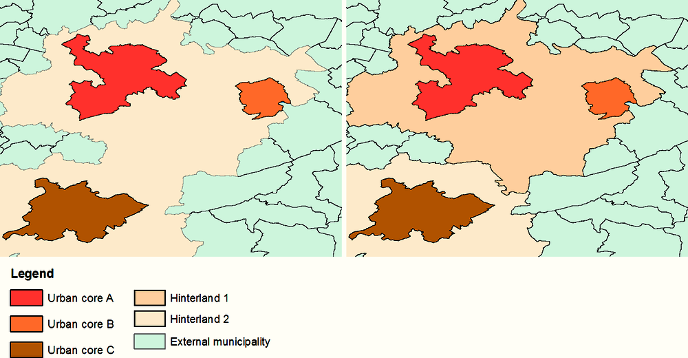
Notes: Left panel: three municipal urban cores grouped into a single functional urban area, assuming that more than 15% of residents in cores B and C commute to core A. Right panel: the same municipal urban cores grouped in two functional urban areas, assuming that: i) less than 15% of core C inhabitants commute to core A and vice versa, ii) less than 15% of core C inhabitants commute to core B and vice versa and iii) at least 15% of population in core A commutes to B and/or vice versa.
Estimating population density across space
The Global Human Settlement (GHS) built-up area dataset (Pesaresi et al., 2015) and the GHS population grid (European Commission, Joint Research Centre (JRC) and Columbia University, Center for International Earth Science Information Network – CIESIN, 2015)6 are used in conjunction with FUA delimitations to compute the indicators proposed in 3.4. The two GHS datasets provide worldwide coverage of development intensity and population density with a high spatiotemporal resolution. The worldwide coverage ensures that the underlying data used to compute the proposed indicators are homogeneous in terms of resolution. This minimises the problem of comparability between indicator values obtained for different geographic units, as they are computed with data of identical spatiotemporal resolution.
The GHS built-up area data (Pesaresi et al., 2015) are provided in raster cells of high resolution (38m × 38m) derived from satellite images.7 The building intensity at each cell is expressed as the fraction of the cell’s surface area, i.e. 1 444 m2 (0.00144 km2), occupied by the footprints of buildings, related structures and civil works. This fraction ranges from zero, when a cell’s surface is estimated to contain no buildings or other structures, to one, which is the case when that surface is estimated to be fully built up. This exercise is illustrated in Figure 3.4. Settlement data display the highest temporal resolution among land-cover datasets available at global scale. The recording of settlement intensity at three time points (1990, 2000, 2014) facilitates the analysis of land-cover changes and the identification of time trends in development intensity.

Notes: Bottom panel: Earth surface. 2nd panel: Earth observation satellites provide images of earth’s surface in the form of raster files. 3rd panel: Extraction of built-up areas, i.e. surface areas covered by buildings and other structures. Top panel: Built-up area raster, expressing the fraction of built-up area in the total size of a grid cell.
Source: Own illustration, based on the presentation of the procedure provided in the GHS website: http://ghslsys.jrc.ec.europa.eu/data.php#GHSLBasics. Satellite photo credit: MaxxL/Wikimedia Commons/CC BY-SA 3.0.

Notes: Bottom panel: Built-up area raster (see also Figure 3.4). 2nd panel: Census data. 3rd panel: Combining census data on population (e.g. at the census tract level) with the built-up area raster. Top panel: Population raster, expressing the number of inhabitants per grid cell.
Source: Own illustration, based on the presentation of the procedure provided in the GHS website: http://ghslsys.jrc.ec.europa.eu/data.php#GHSLBasics.
The GHS population grid dataset (European Commission, Joint Research Centre (JRC) and Columbia University, Center for International Earth Science Information Network – CIESIN, 2015) provides worldwide population density maps. Population data are provided in grid cells of 250 m × 250 m, with the estimated number of inhabitants within each cell surface of 62 500 m2 (0.0625 km2) being reported for 1990, 2000 and 2015. The reported estimates are derived by combining the population figures recorded for administrative areas or census tracts with the high-resolution settlement data derived from satellite images for the same time period. In this context, population estimates for 2015 are combined with built-up area data for 2014. The procedure followed to combine the two datasets is shown in Figure 3.5. A larger development intensity in the underlying settlement grid cells and a larger number of inhabitants in the underlying administrative units imply a larger number of inhabitants allocated to a 250 m × 250 m cell.8
Estimating the spatial distribution of population and built-up land within urban areas
For the computation of the urban sprawl indicators introduced in 3.4, the Global Human Settlement datasets are delimited by each of the FUA boundaries. This procedure is illustrated in Figure 3.6.
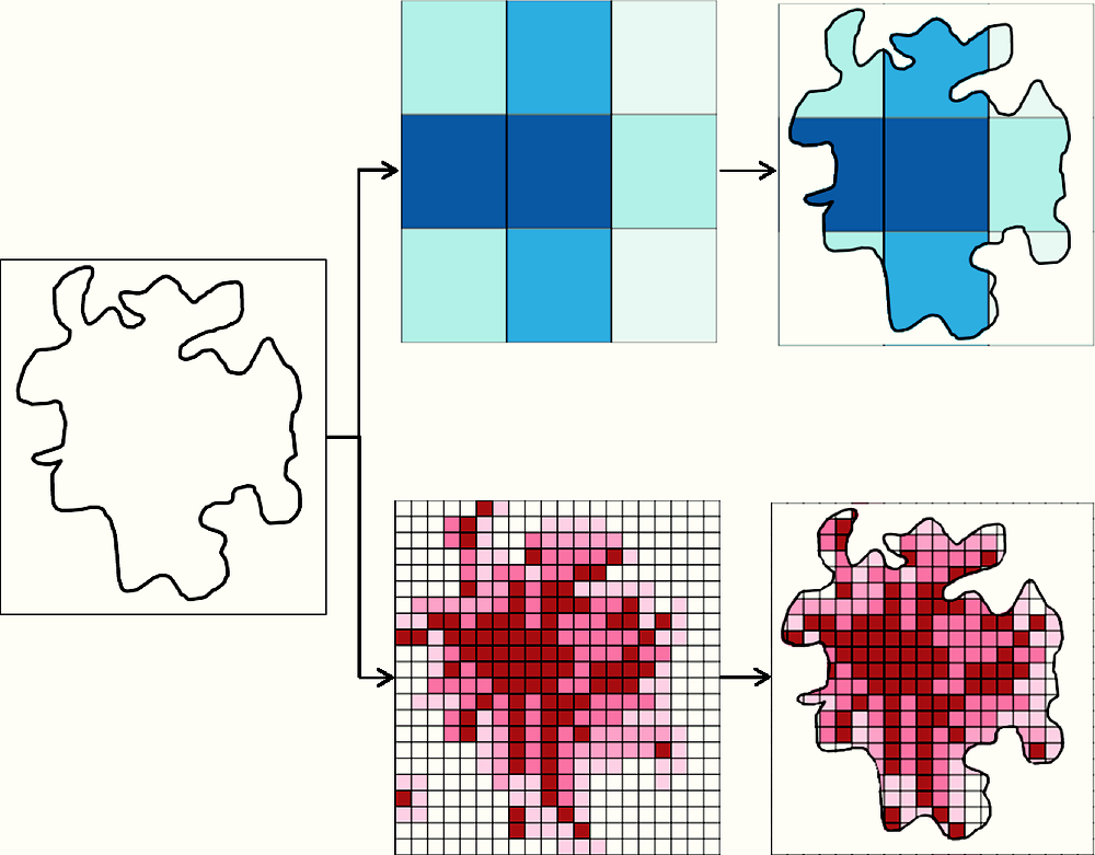
Notes: Left panel: delimitation of a functional urban area (FUA). Upper middle panel: selected cells from population raster map. Lower middle panel: selected cells from a built-up area raster map. Upper right panel: selection of population cells that make up the FUA. Lower right panel: selection of built-up raster cells that make up the FUA.
3.4. Cross-country analyses of urban sprawl indicators
The indicators of urban sprawl used in this study are matched to the urban sprawl dimensions presented in Chapter 2 in Table 3.1. These indicators are selected on the basis of a number of criteria. First, they should enable an analysis of sprawl at certain points in time and facilitate the examination of its changes over time. Second, the different dimensions of sprawl should be conceptually distinct from each other. Third, they should allow for polycentric urban structures, because there is a considerable number of FUAs with more than one centre. The mathematical formulas used for the calculation of each indicator at the FUA level, as well as those used for aggregating the city-level indicators to the country level, are presented in Appendix 3.A.
This section provides static and intertemporal cross-country comparisons based on these indicators. Static comparisons are performed using average values at the country level for the year 2014, which is referred to as the current situation. In addition, the provided cross-country comparisons report the FUAs in which indicators obtain their minimum and maximum values in each country. This facilitates a visual inspection of the range of values taken by different indicators across the FUAs of a country.
On the other hand, intertemporal comparisons are entirely based on the evolution of indicator values at the country level, which are obtained for 29 countries (all OECD member countries, except for Estonia, Iceland, Israel, Latvia, New Zealand and Turkey) in three time points: 1990, 2000 and 2014.9 Countries are ranked according to the total change occurred between 1990 and 2014. The changes that took place in the periods 1990-2000 and 2000-14 are displayed together with the corresponding total changes. All changes are computed and reported in absolute terms.
Average urban population density
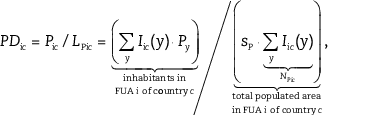
The average population density of an urban area is the average number of inhabitants per km2 of populated urban space. This is the ratio of the urban area’s total population to the total inhabited surface within that urban area. The indicator is computed at the urban area level using Equation (1) in Appendix 3.A. The value of the indicator at the country level is computed using Equation (2) of the appendix and is equivalent to the average population density that would be observed had all FUAs of the country been concatenated in a single urban area.
Current situation
Statistics of the average population density of urban areas for the 29 OECD countries included in the study are provided in Figure 3.7. Countries are ranked from highest to lowest mean of average population density levels in 2014. The figure also displays the minimum and maximum values of average population density at the FUA level and the names of the corresponding urban areas.
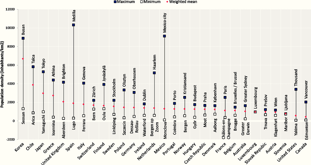
Notes: Red diamond-shaped points indicate average urban population densities at the country level. Minimum and maximum values of the indicator at the city level are indicated with white and blue squares respectively.
Source: Own calculations, based on GHS built-area data (Pesaresi et al., 2015), GHS population data (European Commission, Joint Research Centre (JRC) and Columbia University, Center for International Earth Science Information Network – CIESIN, 2015) and FUA delimitations (OECD, 2012).
As revealed by the ranking of countries, urban areas of Canada and the United States are, on average, the least dense. However, urban areas of both countries are heterogeneous and display average densities that lie in a wide range. Specific functional urban areas, such as New York and Vancouver, have an average population density that exceeds the average density observed in most European cities. For example, Vancouver is much denser than Copenhagen or Prague, despite urban areas of Denmark and Czech Republic being on average much denser than those of Canada. On the other hand, the least dense FUAs in these countries display densities that fall below the threshold of 150 people per km2, which is the threshold used to define rural areas (OECD, 2011). To ensure that country mean densities are not affected by outlier values, North American functional urban areas with a density below 80 inhabitants per km2 were excluded from the study.10
The average population density of urban areas obtains values between 1 000 and 2 000 people per km2 for the majority of countries. However, within-country variation is remarkably high, primarily across urban areas of Mexico and Spain, and secondarily of Korea, The Netherlands and Chile. Greece and the United Kingdom are the only European countries where density of urban areas exceeds the threshold of 2 000 people per km2. The figure also reveals that urban areas in Korea and Japan are, on average, some of the densest worldwide. However, both countries contain diverse urban areas with local averages that vary widely, peaking in the cities of Busan and Tokyo respectively. Chile is the second densest country among the ones analysed here, with the majority of its urban areas being very dense.
Trends 1990-2014
The evolution of average urban population density between 1990 and 2014 in the 29 OECD countries is displayed in Figure 3.8.11 The figure also shows how this total change is decomposed into changes occurring during the two sub-periods of 1990-2000 and 2000-14. A negative change implies that the populated footprint occupied by the urban areas of a country grew faster than its population in that period, whereas a positive change implies the opposite.
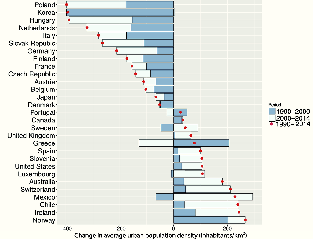
Notes: Red dots represent the total change in average urban population density in the period 1990-2014. The bars decompose the total change into changes occurring during the periods 1990-2000 (darker blue) and 2000-14 (lighter blue).
Source: Own calculations, based on GHS built-area data (Pesaresi et al., 2015), GHS population data (European Commission, Joint Research Centre (JRC) and Columbia University, Center for International Earth Science Information Network – CIESIN, 2015) and FUA delimitations (OECD, 2012).
Since 1990, average urban population density has increased in 15 countries and has declined in 14. Despite density having increased in most of the countries, reductions of urban population density are, on average, much larger than relevant increases. This is mainly due to important reductions of population density in several countries, such as Korea and Italy, during the period 1990-2000. The most important reductions of average urban population density are observed in Poland, Korea, Hungary and the Netherlands. In Korea, the large decline of population density in the period 1990-2000 was followed by a minor increase in density in the period 2000-14. On the other hand, in Germany and the Slovak Republic, a relatively large share of the density decline has occurred after 2000.
The largest increases of average urban population density since 1990 have occurred in Norway, Ireland, Chile and Mexico. These increases have mainly occurred after 2000 (except for Norway), with Mexico showing the greatest increase in absolute terms among the examined countries in the period 2000-14. Average urban population density has increased in all three countries with the lowest density in 2014: Slovenia, United States and Canada. In Greece and Portugal, densification of the period 1990-2000 was slightly reversed in the period 2000-14, when urban population density declined in both countries.
Population-to-density allocation
The allocation of population to areas of relatively low density is captured by the share of population living in areas where density is below a certain threshold. Three thresholds are considered in this report: 1 500, 2 500 and 3 500 inhabitants per km2. The lower threshold of 1 500 people per km2 matches the threshold value used by the OECD (2012) to identify areas which can be considered as urban. Under the conditions presented in 3.3 such areas make up the urban cores, the fundamental building block of a functional urban area. The higher threshold of 3 500 people per km2 is based on the study by Newman and Kenworthy (2006). Using data from 58 higher-income cities, that study suggests the existence of a critical urban density threshold, placed at approximately 3 500 inhabitants (or workers) per km2, above which car dependency is significantly reduced. Finally, the middle threshold of 2 500 people per km2 is a natural intermediate step between the other two values. It should also be mentioned that areas with population density up to 150 inhabitants per km2 are not considered in the calculation of the indicator, as this is the threshold below which areas are considered as rural (OECD, 2011).
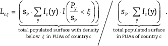
At the city level, the share of population living in areas of the FUA where density lies below one of the three aforementioned thresholds is computed using Equation (3) in Appendix 3.A. At the country level, the indicator reflects the share of urban population residing in areas of all FUAs of the country where density is below the selected threshold. This indicator is calculated using Equation (4) in Appendix 3.A. In the cross-country analysis of the indicator that follows, the selected threshold is the lowest of the ones presented above, i.e. 1 500 inhabitants per km2.
Current situation
The statistics associated with the share of population residing in areas where density is between 150 and 1 500 people per km2 are provided in Figure 3.9. The 29 countries considered in the report are ranked, from highest to lowest, with respect to the share of their urban population that was residing in such areas in 2014. The figure also displays the minimum and maximum values obtained by the indicator at the FUA level, as well as the names of the corresponding urban areas.
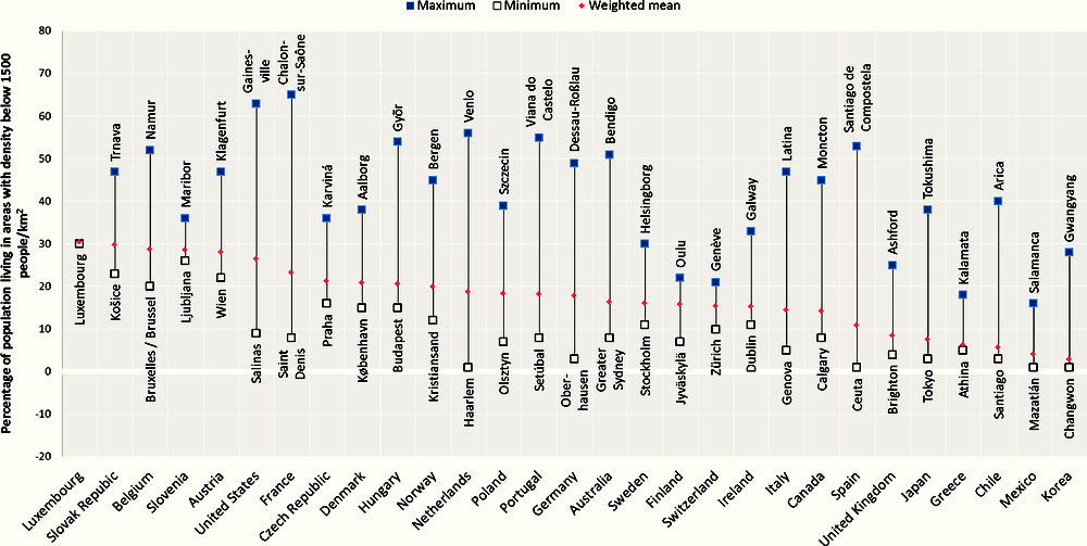
Notes: Red diamond-shaped points indicate the average share of population residing in areas with density of 150-1 500 inhabitants/km2 at the country level. Minimum and maximum values of the indicator at the city level are indicated with white and blue squares respectively.
Source: Own calculations, based on GHS built-area data (Pesaresi et al., 2015), GHS population data (European Commission, Joint Research Centre (JRC) and Columbia University, Center for International Earth Science Information Network – CIESIN, 2015) and FUA delimitations (OECD, 2012).
The resulting ranking of countries differs substantially from the cross-country ranking of average population density provided in Figure 3.7. First, the countries with the lowest urban population density are not found at the top of the ranking. For instance, less than 15% of the urban population of Canada resides in areas of very low population density, a value that lies far below the maximum recorded in Luxemburg (30.5%). Second, countries with moderate levels of average population density can be found at the lower end of the ranking. For instance, only a very small portion of Mexico’s urban population resides in locations where density lies between 150 and 1 500 inhabitants per km2. Korea, Chile, Greece and Japan score similarly in both indicators in 2014: their urban areas are dense and only a very low share of their population resides in those parts of their FUAs where density is very low.
Trends 1990-2014
The intertemporal changes in the percentage of population residing in areas of very low population density (150-1 500 inhabitants per km2) for the 29 OECD countries considered in the analysis are displayed in Figure 3.10. The total change between 1990 and 2014, which is denoted by dots, is also decomposed into changes occurring during the two sub-periods: 1990-2000 and 2000-14.
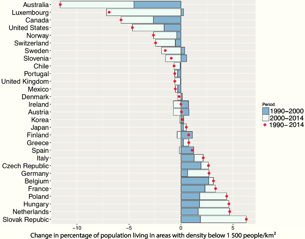
Notes: Red dots represent the total change in the share of population residing in areas with density of 150-1 500 inhabitants/km2 in the period 1990-2014. The bars decompose the total change into changes occurring during the periods 1990-2000 (darker blue) and 2000-14 (lighter blue).
Source: Own calculations, based on GHS built-area data (Pesaresi et al., 2015), GHS population data (European Commission, Joint Research Centre (JRC) and Columbia University, Center for International Earth Science Information Network – CIESIN, 2015) and FUA delimitations (OECD, 2012).
Overall, the share of population living in areas of very low density has increased in about half of the countries. The largest increase of the indicator is observed in Slovak Republic (about 6 percentage points), followed by the Netherlands, Hungary and Poland. On the other hand, the largest decline of the share of population living in areas of very low density since 1990 occurred in the urban areas of Australia (about 12 percentage points), Luxembourg, Canada and the United States. In all countries mentioned above, a major part of the observed changes has occurred in more recent years, i.e. during the period 2000-14.
The increases of the indicator displayed in Figure 3.10 may be driven by different forces. First, the indicator may have increased because some low-density areas (150-1 500 inhabitants/km2) have densified without their density exceeding the threshold of 1 500 inhabitants per km2. Another reason for the observed increases may be that new areas that were previously undeveloped are converted to low-density locations or that density decreases in areas where it has previously been slightly above 1 500 inhabitants per km2. To identify whether the evolution of the indicator is driven by the latter type of change, the values of the population-to-density allocation indicator should be examined in conjunction with the corresponding values of the land-to-density allocation indicator, which is provided in Figures 3.11 and 3.12 below.
Another important insight provided by Figure 3.10 is that in a few European countries, such as Greece and Spain, both average urban population density and the percentage of population residing in areas with population density of 150-1 500 inhabitants per km2 have increased. This finding indicates that in some of the urban areas of these countries densification has been accompanied by suburbanisation. This phenomenon is examined in more detail separately for each country in the sheets available in Appendix 3.B.
Land-to-density allocation
The allocation of urban land to areas of relatively low density is captured by the share of urban land occupied by areas where density lies below a certain threshold. As with the population-to-density allocation, the thresholds considered are 1 500, 2 500 and 3 500 inhabitants per km2 (for the rationale behind selecting these thresholds, see the relevant discussion in the presentation of the population-to-density allocation). At the city level, the share of land occupied by areas where density lies below a threshold value is computed using Equation (5) in Appendix 3.A. At the country level, the indicator reflects the share of urban land occupied by areas of all FUAs of the country where density is below the selected threshold. This indicator is calculated using Equation (6) in Appendix 3.A. In the cross-country analysis of the indicator that follows, the selected threshold is the lowest of the ones presented above, i.e. 1 500 inhabitants per km2.
Current situation
Statistics of the share of urban land (footprint) occupied by areas in which population density is between 150 and 1 500 inhabitants per km2 for the 29 OECD countries analysed here are provided in Figure 3.11. Countries are ranked from highest to lowest average share of urban land (footprint) with such population densities at the country level in 2014. The figure displays the minimum and maximum values of the indicator at the FUA level, and the names of the corresponding urban areas.
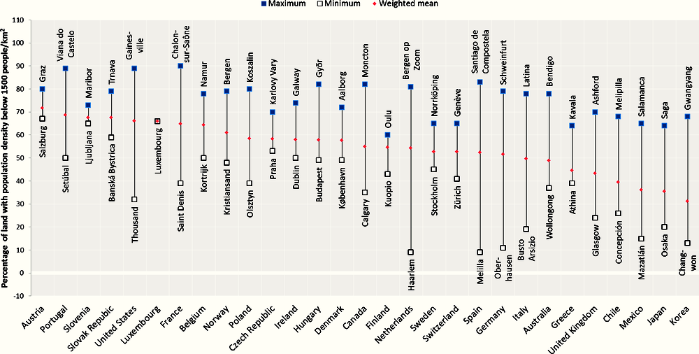
Notes: Red diamond-shaped points indicate the average share of urban footprint with density of 150-1 500 inhabitants/km2 at the country level. Minimum and maximum values of the indicator at the city level are indicated with white and blue squares respectively.
Source: Own calculations, based on GHS built-area data (Pesaresi et al., 2015), GHS population data (European Commission, Joint Research Centre (JRC) and Columbia University, Center for International Earth Science Information Network – CIESIN, 2015) and FUA delimitations (OECD, 2012).
In many respects, the ranking resembles that of the share of population residing in areas of very low density, displayed in Figure 3.9, with the same set of six countries found in the lower end of the two rankings (even though in a different order). That is, functional urban areas in Korea, Japan, Mexico, Chile, United Kingdom and Greece contain the smallest percentages of land exposed to very low density levels, all below 45%. On the other hand, the national average values in Belgium, France, Luxembourg, United States, Slovak Republic, Slovenia and Austria all lie above 64%.
The share of urban footprint occupied by areas where population density is very low is strongly correlated with the share of population residing in areas of such density levels, but the two indicators provide complementary information.12 This is highlighted in the case of Portugal, where the share of population residing in areas of very low density is modest, i.e. about 18%, but the share of urban footprint occupied by areas of very low density obtains the second largest value recorded in the national ranking, i.e. about 69%. Such a large divergence can mainly be attributed to a considerably lower population density in areas with less than 1 500 inhabitants per km2 than the one in areas where density exceeds that threshold. In case of such large differences between the two indicators, population density is likely to display a large variation across the urban surfaces of a country. The analysis of the next indicator (variation of population density) supports this hypothesis.
Trends 1990-2014
The intertemporal changes in the share of urban footprint hosting areas of population density below 1 500 inhabitants per km2 for the 29 OECD countries are presented in Figure 3.12. The total change between 1990 and 2014, which is denoted by the red dots, is also decomposed into changes occurring during the two sub-periods: 1990-2000 and 2000-14. In the majority of countries, the share of urban footprint in very low density areas increased since 1990, with the largest growth recorded in Hungary (9 percentage points), the Netherlands, Belgium, Germany and Poland. On the other hand, the largest reductions are recorded in Australia (10 percentage points), the United States and Canada. To a large extent, these changes reflect the evolution of the share of population residing in areas of very low density in the aforementioned countries, shown in Figure 3.10.13
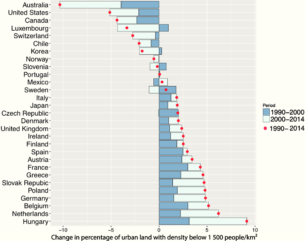
Notes: Red dots represent the total change in the share of urban footprint with density of 150-1 500 inhabitants/km2 in the period 1990-2014. The bars decompose the total change into changes occurring during the periods 1990-2000 (darker blue) and 2000-14 (lighter blue).
Source: Own calculations, based on GHS built-area data (Pesaresi et al., 2015), GHS population data (European Commission, Joint Research Centre (JRC) and Columbia University, Center for International Earth Science Information Network – CIESIN, 2015) and FUA delimitations (OECD, 2012).
In some countries, especially in Europe (Greece, Ireland, Spain, Sweden and the United Kingdom), both average urban population density and the percentage of urban footprint occupied by areas of very low density (150-1 500 inhabitants per km2) have increased. This reflects that in some of the urban areas of these countries densification has co-evolved with suburbanisation. However, this trend is also observed in cities of other countries. Box 3.1 displays the case of Santiago, the capital of Chile, whose functional urban area experienced both a growth in average population density and an increase in the share of urban land allocated to very low density levels (150-1 500 inhabitants per km2) between 1990 and 2014.
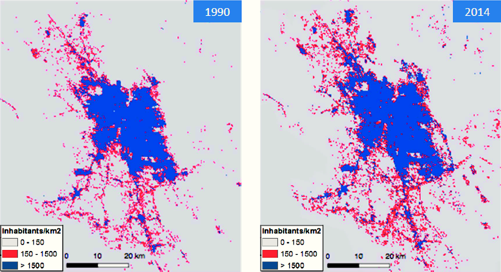
Notes: Left panel: Distribution of population density across three intervals (< 150, 150-1 500, and > 1 500 inhabitants per km2) in Santiago in 1990. Right panel: Distribution of population density across the same intervals in 2014.
The coevolution of densification and suburbanisation over time is reflected well in the case of Santiago. Back in 1990, the average population density in the parts of the functional urban area hosting more than 150 inhabitants per km2 (the coloured parts in the figure on the left) was approximately 5 606 inhabitants per km2. In the same year, roughly 29% of that surface was hosting densities below 1 500 inhabitants per km2. That area is represented by the red pixels of the figure.
The urban area of Santiago expanded significantly in the period from 1990 to 2014, as indicated by the difference in the number of coloured surfaces between the two panels. While average density in the areas represented by these coloured surfaces increased by 2.2% between 1990 and 2014, the composition of developed land changed in favour of low-density areas. By 2014, the share of developed land hosting density levels below 1 500 inhabitants per km2 (red pixels) had increased by 3.3%, while the share of population residing in areas of such density had increased by 4.2%. This is depicted in the growth of red pixels, which is faster than the growth of blue pixels in the examined period.
Source: Own elaboration, based on GHS built-area data (Pesaresi et al., 2015), GHS population data (European Commission, Joint Research Centre (JRC) and Columbia University, Center for International Earth Science Information Network – CIESIN, 2015) and FUA delimitations (OECD, 2012).
Variation of urban population density
Population density often varies substantially among different areas of a city. The indicator used to measure the level of variation of urban population density is the coefficient of variation (also known as relative standard deviation). At the city level, the indicator is equal to the ratio of the standard deviation of population density in an FUA over the mean of population density in that FUA. The mathematical formula used to compute the coefficient of variation at the city level is presented in Equation (8) of Appendix 3.A. At the country level, the indicator shows the ratio of the standard deviation of population densities at all locations in the FUAs of a country from the national mean of urban population density over that mean. The indicator at the country level is calculated using Equation (10) of Appendix 3.A.
Current situation
The statistics associated with the variation of urban population density for the 29 OECD countries are provided in Figure 3.13. Countries are ranked from highest to lowest coefficient of variation of urban population density at the country level in 2014. The figure also displays the minimum and maximum values of the coefficient of variation at the FUA level and the names of the corresponding urban areas.
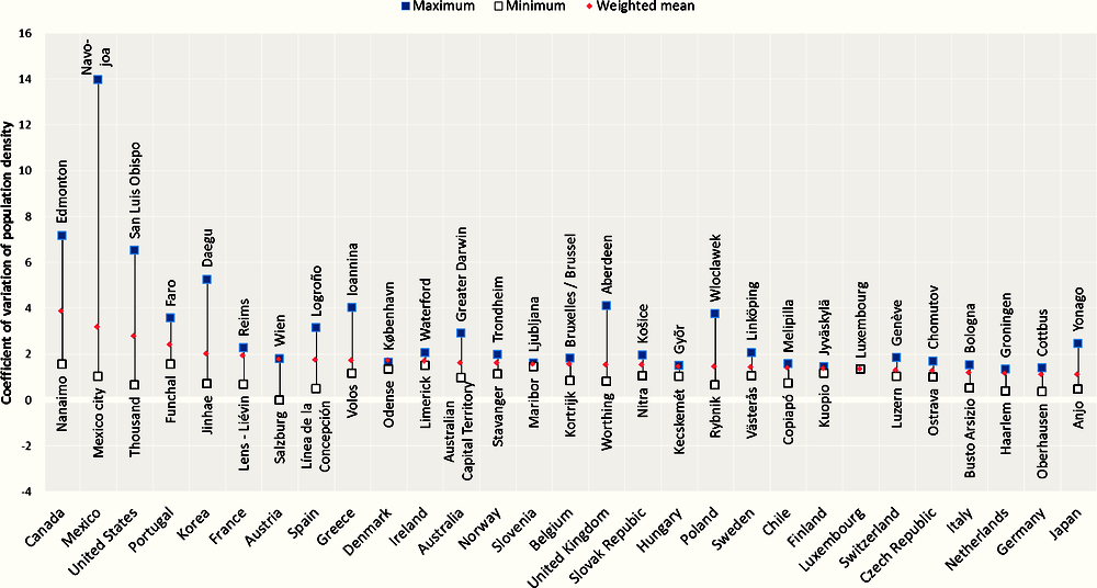
Notes: Red diamond-shaped points indicate the average coefficient of variation of urban population density at the country level. Minimum and maximum values of the indicator at the city level are indicated with white and blue squares respectively.
Source: Own calculations, based on GHS built-area data (Pesaresi et al., 2015), GHS population data (European Commission, Joint Research Centre (JRC) and Columbia University, Center for International Earth Science Information Network – CIESIN, 2015) and FUA delimitations (OECD, 2012).
Urban areas of Canada, Mexico and the United States are characterised, on average, by the largest coefficient of variation among the examined OECD countries. However, urban areas of these countries are heterogeneous, thus the coefficient values at the FUA level range widely across cities. On the other hand, the lowest variation of urban population density is observed in The Netherlands, Germany and Japan.
The relationship between the mean and the coefficient of variation of urban population density at the country level is not particularly strong. Indeed, cities in countries including Chile, Finland, Italy, Japan and Switzerland are dense and have a relatively low coefficient of variation of density, and urban areas in Canada, France and the United States are rather sparsely populated and have a high coefficient of variation of density. However, countries may be placed closer to the lower end in the coefficient of variation ranking while their average urban population density is also relatively low. For instance, Luxembourg and the urban areas of Czech Republic have relatively low population density but are, on average, also among the ones with the lowest coefficient of variation across OECD countries. On the other hand, the coefficient of variation is relatively high in Korea, Greece and Spain, despite these countries ranking high in terms of average urban population density.
Trends 1990-2014
The intertemporal changes of the coefficient of variation of urban population density for the 29 studies included in the analysis are shown in Figure 3.14. The total change between 1990 and 2014, which is denoted by the red dots, is also decomposed into changes occurring during the two sub-periods: 1990-2000 and 2000-14, denoted by bars of different colours.
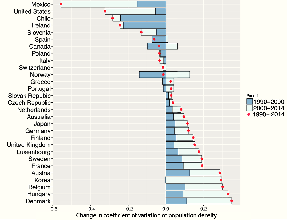
Notes: Red dots represent the total change in the coefficient of variation of urban population density at the country level in the period 1990-2014. The bars decompose the total change into changes occurring during the time periods 1990-2000 (darker blue) and 2000-14 (lighter blue).
Source: Own calculations, based on GHS built-area data (Pesaresi et al., 2015), GHS population data (European Commission, Joint Research Centre (JRC) and Columbia University, Center for International Earth Science Information Network – CIESIN, 2015) and FUA delimitations (OECD, 2012).
The variation of urban population density has increased over time in most of the countries included in the analysis. In absolute terms, increases in the coefficient of variation since 1990 have been particularly high in Denmark, Hungary, Belgium, while the largest increase since 2000 is observed in Korea. On the contrary, variation of urban population density has declined sharply in Mexico, especially since 2000. The United States, Chile and Ireland have also seen large reductions in the variation of urban population density in the period 1990-2014.
Fragmentation
The fragmentation index measures the number of urban fabric fragments per km2 of built-up area. At the city level, the indicator is computed using Equation (11) of Appendix 3.A. At the country level, the fragmentation index is obtained by dividing the total number of fragments identified in all functional urban areas of the country by the total amount of artificial land in the same areas. The formula used to compute the indicator at the country level is provided in Equation (12) of the same appendix.
Current situation
Statistics of the fragmentation of urban fabric for the 29 OECD countries analysed here are provided in Figure 3.15. Countries are ranked from highest to lowest average fragmentation of urban fabric in 2014. The figure also displays the minimum and maximum values of fragmentation at the FUA level and the names of the corresponding urban areas.
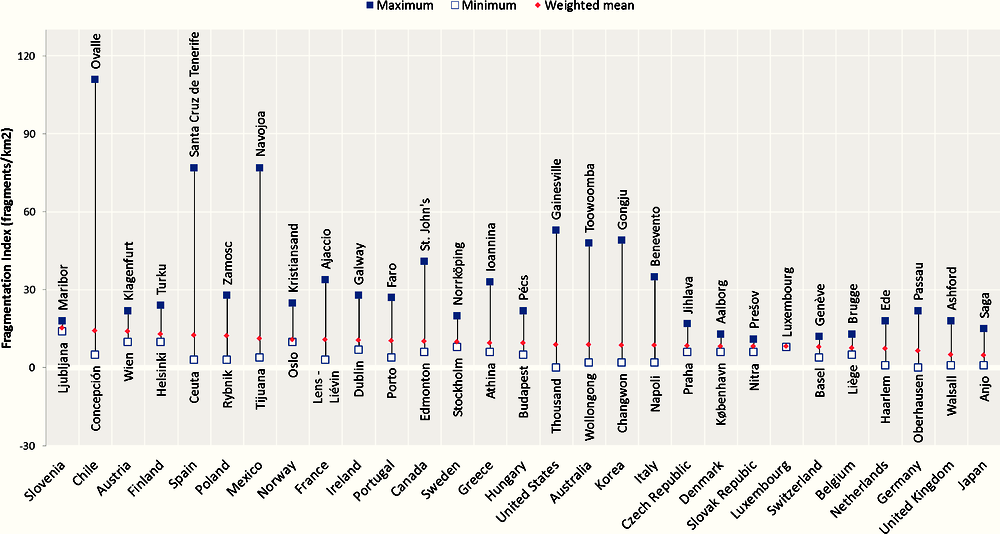
Note: Red diamond-shaped points indicate average fragmentation of urban fabric at the country level. Minimum and maximum values of the indicator at the city level are indicated with white and blue squares respectively.
Source: Own calculations, based on GHS built-area data (Pesaresi et al., 2015) and FUA delimitations (OECD, 2012).
In 2014, fragmentation at the country level ranged from 4.91 fragments per km2 of artificial area in Japan to around 15.21 in Slovenia. Fragmentation is relatively high in the urban areas of Chile, Austria and Finland and relatively low in the urban areas of the United Kingdom, Germany and the Netherlands. The within-country variation of the indicators, i.e. the variation of fragmentation among cities of the same country, is very high. That is, in many cases the value of the fragmentation index at the country level lies far below the values recorded in multiple FUAs of a given country. On the other hand, large metropolitan areas usually exhibit rather low levels of fragmentation, as the fragmentation index in these areas is often found to lie below the corresponding index at the country level.
The relationship between fragmentation of urban fabric and urban population density does not turn out to be particularly strong at the country level. On the one hand, urban areas in countries including Japan, the United Kingdom and Switzerland are both dense and not very fragmented, and areas in Austria and Slovenia are both fragmented and sparsely populated. On the other hand, cities in Belgium, Luxembourg and Slovak Republic display relatively low population density, but also quite low fragmentation. Other examples are Chile and Spain, where urban fabric is rather fragmented, despite these countries ranking high in terms of average urban population density.
Trends 1990-2014
The evolution of fragmentation of urban fabric over time for the 29 countries considered in the analysis is provided in Figure 3.16. The total change in the average number of fragments per km2 of artificial area between 1990 and 2014, which is denoted by the red dots, is also decomposed into changes occurring during the two sub-periods: 1990-2000 and 2000-14, denoted by bars of different colours.
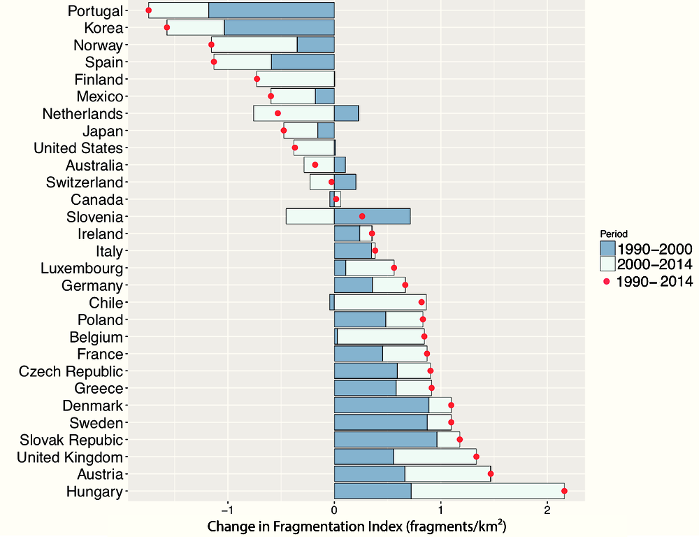
Note: Red dots represent the total change in fragmentation of urban fabric at the country level in the period 1990‐2014. The bars decompose the total change into changes occurring during the time periods 1990-2000 (darker blue) and 2000-14 (lighter blue).
Source: Own calculations, based on GHS built-area data (Pesaresi et al., 2015) and FUA delimitations (OECD, 2012).
Fragmentation has increased in 18 of the 29 countries included in the analysis since 1990. The largest increases are recorded in Hungary (more than two fragments per km2), Austria, the United Kingdom and Slovak Republic, while increases of more than one fragment per km2 have been recorded in Denmark and Sweden. Fragmentation has also increased significantly in Chile and Belgium from 2000 onwards. By contrast, the largest decreases in fragmentation since 1990 are observed in Portugal (about 1.7 fragments per km2), Korea, Norway and Spain (all by more than one fragment per km2). The largest decline of fragmentation in the period 2000-14 has been recorded in Norway, the Netherlands and Finland.
Polycentricity
The polycentricity indicator is defined as the number of urban centres, i.e. the number of population-density peaks in an urban area. The approach followed to identify these centres is explained in detail in Appendix 3.A. At the country level, the polycentricity index is computed by dividing the total number of high-density peaks identified in the FUAs of a country by the total number of FUAs in that country.
Current situation
The statistics of polycentricity for the 29 OECD countries considered in the report are provided in Figure 3.17. Countries are ranked, from highest to lowest, according to the average number of centres identified in their FUAs in 2014. The figure also displays the minimum and maximum values of fragmentation at the FUA level and the names of the urban areas attaining the maximum values.
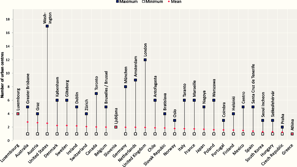
Note: Red diamond-shaped points indicate the average number of peaks of urban population density at the country level. Minimum and maximum values of the indicator at the city level are indicated with white and blue squares respectively. A minimum value of one implies that at least one urban area in the country has been found to be monocentric. Cities corresponding to minimum values are not reported since in most countries the minimum value of one applies to multiple cities. All urban areas in Slovenia are found to have two centres. All urban areas in Greece are found to be monocentric. Country averages are not weighted, i.e. dots represent the expected number of centres in a randomly selected urban area of a country.
Source: Own calculations, based on GHS built-area data (Pesaresi et al., 2015), GHS population data (European Commission, Joint Research Centre (JRC) and Columbia University, Center for International Earth Science Information Network – CIESIN, 2015) and FUA delimitations (OECD, 2012).
Urban areas with multiple density peaks are identified in every country, apart from Greece, where all FUAs were found to be monocentric. Both FUAs of Slovenia have two density peaks (centres) and the only FUA in Luxembourg has four. The range in the rest of the countries varies between one and a maximum which is often observed in the country’s largest urban area (e.g. Brussels in Belgium, Toronto in Canada, Copenhagen in Denmark, Helsinki in Finland, Dublin in Ireland, Amsterdam in the Netherlands, Oslo in Norway, Warsaw in Poland and London in the United Kingdom, Washington in the United States) or in one of the biggest FUAs (Greater Brisbane in Australia, Graz in Austria, Marseille in France, Munich in Germany, Gothenburg in Sweden). The highest average numbers of urban centres after Luxembourg are observed in Australia, Austria and the United States, whereas the lowest ones after Greece are recorded in Czech Republic, Hungary and Korea.
Trends 1990-2014
Intertemporal changes in the average number of peak-density points in the FUAs of OECD countries are presented in Figure 3.18. The total change of the indicator between 1990 and 2014, which is denoted by the red dots, is also decomposed into changes occurring during the two sub-periods: 1990-2000 and 2000-14, denoted by bars of different colours.
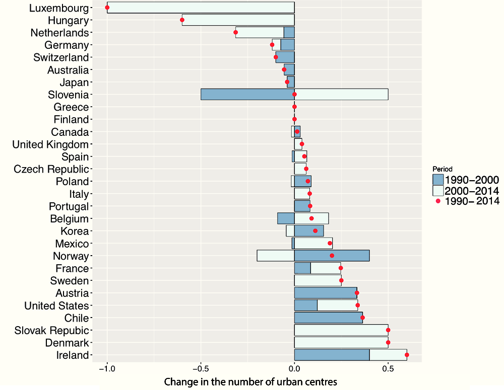
Note: Red dots represent the total change in the polycentricity index at the country level in the period 1990-2014. The bars decompose the total change into changes occurring during the time periods 1990-2000 (darker blue) and 2000-14 (lighter blue).
Source: Own calculations, based on GHS built-area data (Pesaresi et al., 2015), GHS population data (European Commission, Joint Research Centre (JRC) and Columbia University, Center for International Earth Science Information Network – CIESIN, 2015) and FUA delimitations (OECD, 2012).
The number of urban centres (urban peak-density points) has increased in the majority of countries since 1990. Some of the largest increases in this number are observed in Ireland, Denmark, Slovak Republic and Chile. In these countries, population density has adjusted in a way that new urban centres have emerged within existing urban areas. Since 2000, the greatest increases have been recorded in Denmark, the Slovak Republic and Slovenia, where a new urban centre has emerged in every second urban area of the country. However, it is important to note that the magnitude of the changes observed in Slovenia and Luxembourg, where the indicator declined by one urban centre since 2000, could be partially attributed to the fact that the two countries contain only one and two FUAs respectively. Following Luxembourg, the largest decreases of polycentricity have occurred in Hungary, the Netherlands and Germany.
Decentralisation
The decentralisation index shows the share of urban population residing outside of the urban centres of a FUA. The approach followed to identify urban centres in each FUA is described in detail in Appendix 3.A. The mathematical formula used to compute decentralisation at the city level is provided in Equation (15) of the appendix. At the country level, the indicator reflects the share of urban population residing outside of all urban centres of the FUAs of a country. This share is computed using Equation (16) in Appendix 3.A.
Current situation
The statistics associated with decentralisation, i.e. the share of urban population residing outside FUA centres, for the 29 OECD countries considered in the analysis are provided in Figure 3.19. Countries are ranked according to the values of the decentralisation index recorded for 2014, from highest to lowest. The figure also displays the minimum and maximum values of the decentralisation indicator at the FUA level, as well as the names of the corresponding urban areas.14

Note: Red diamond-shaped points indicate the average fraction of urban population residing outside FUA centres at the country level. Minimum and maximum values of the indicator at the city level are indicated with white and blue squares respectively.
Source: Own calculations, based on GHS built-area data (Pesaresi et al., 2015), GHS population data (European Commission, Joint Research Centre (JRC) and Columbia University, Center for International Earth Science Information Network – CIESIN, 2015) and FUA delimitations (OECD, 2012).
Average decentralisation in urban areas varies substantially across OECD countries, with values ranging from 19% in Greece to 37% in Slovenia. Following Slovenia, decentralisation is highest in the Slovak Republic, Belgium, and Luxembourg, where the percentage of population living outside FUA centres is 35% or higher. The average share of urban population residing outside FUA centres in the 29 countries considered in the analysis is about 30%. Greece, Korea, Chile and Mexico are the only countries in which that percentage lies below 25%.
Trends 1990-2014
Intertemporal changes in the average fraction of population residing outside urban centres, but still within FUA boundaries of OECD countries, are presented in Figure 3.20. The total change of the decentralisation indicator between 1990 and 2014, which is denoted by the red dots, is also decomposed into changes occurring during the two sub-periods: 1990‐2000 and 2000-14, denoted by bars of different colours.
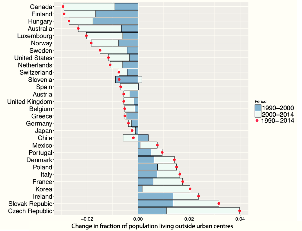
Note: Red dots represent the total change in the decentralisation index at the country level in the period 1990-2014. The bars decompose the total change into changes occurring during the time periods 1990-2000 (darker blue) and 2000-14 (lighter blue).
Source: Own calculations, based on GHS built-area data (Pesaresi et al., 2015), GHS population data (European Commission, Joint Research Centre (JRC) and Columbia University, Center for International Earth Science Information Network – CIESIN, 2015) and FUA delimitations (OECD, 2012).
In contrast to most other indicators of urban sprawl developed in this study, decentralisation has declined in the majority of countries since 1990. It has only grown in 10 countries, with the largest increases observed in Czech Republic (about 4 percentage points increase), Slovak Republic, Ireland and Korea.15 In the rest of the countries where decentralisation increased, its growth was lower than 2 percentage points. On the other hand, the strongest centralisation forces in the period 1990-2014 are observed in Canada (about 4 percentage points decline), Finland, Hungary and Australia. It is also noteworthy that the separate changes that took place during the two sub-periods (1990-2000 and 2000-14) point to the same direction (positive or negative) for all countries analysed here except for Chile, Slovenia and Spain.
3.5. Country-level analysis
This section presents the main findings from the analysis of the current state of urban sprawl and its evolution over time for each country separately. A detailed presentation of that analysis is provided in the country sheets of Appendix 3.B, which contain one-page summaries of the state and evolution of urban sprawl for each of the 29 countries analysed here.
The country-level analysis reveals that urban areas in some countries in Central Europe and North America, such as Austria and Slovenia, and Canada and the United States, are among the most sprawled ones. This is manifested in their high rank in most dimensions of urban sprawl. Cities in Canada and the United States are on average more sparsely populated than cities in these European countries, and urban population density varies much more within them.
Another small group of countries score low in most dimensions of urban sprawl. Greece, Japan, Korea and the United Kingdom are at the bottom of the ranking of multiple indicators of sprawl. Chile, Mexico and Spain also seem to perform well in multiple dimensions of sprawl, but their urban areas are still relatively fragmented.
Focusing on the evolution of urban areas over time, cities in Denmark, France, and several Central European countries, such as Czech Republic, Hungary, Poland and Slovak Republic have sprawled along most of the dimensions examined since 1990. On the other hand, urban sprawl has declined in Australia, Spain and Switzerland, where urban areas have become much denser and less fragmented than they were in 1990. Cities have also become denser and less fragmented in Canada and the United States, which were characterised, however, by the lowest levels of density in both 1990 and 2014.
3.6. Summary
This chapter operationalised and measured urban sprawl, as the latter was conceptualised in Chapter 2. The seven indicators used to characterise the different dimensions of urban sprawl have been computed for 1 156 urban areas in 29 OECD countries and for different time points (1990, 2000, 2014) thanks to newly released datasets that follow the evolution of artificial surfaces and population density worldwide. The indicators have then been used to conduct cross-city, cross-country and country-level analyses of urban sprawl.
Urban population density has declined, on average, in 14 of the 29 OECD countries examined here between 1990 and 2014. Some of these countries contained relatively dense areas in 1990. In 2014, urban areas in Korea, Chile, Japan and Greece were the densest and those of Canada, the United States and Slovenia were the least dense among the examined OECD countries.
Interesting insights are also provided by the analysis of two new measures of sprawl: the share of developed surfaces hosting residential areas of low density, and the share of urban population residing in those areas. The analysis revealed that the sharp decline in average population density observed in many OECD countries between 1990 and 2014 was driven by rapid suburbanisation. This is indicated by a substantial increase of the share of urban developed surfaces hosting residential areas of very low density, i.e. 150-1 500 inhabitants per km2, observed in that period. However, in some countries (Greece, Ireland, Spain, Sweden and the United Kingdom) both average urban population density and the percentage of urban footprint occupied by areas of very low density (150-1 500 inhabitants per km2) have increased. This shows that in some of the urban areas of these countries densification coincided with the above suburbanisation process, either because initial urban population density was, on average, very low or because population in already dense parts of urban space increased even further.
At the same time, the relationship between urban population density and fragmentation is not particularly strong at the country level. For example, fragmentation of urban areas in Chile and Spain is relatively high, whereas cities in these countries are among the densest of those analysed. Decentralisation is highest in urban areas of Slovenia, Slovak Republic, Belgium, and Luxembourg, where the percentage of population living outside the urban core exceeds 35%. Greece, Korea, Chile and Mexico are the only countries where that percentage lies below 25%.
Some countries, including Austria and Slovenia rank relatively high in most dimensions of urban sprawl. Other countries, such as Canada and the United States, are very sparsely populated, but score lower in indicators of fragmentation and decentralisation. Looking at the evolution of cities since 1990, urban areas in Czech Republic, Denmark, France, Hungary, Poland and Slovak Republic have been sprawling along most of the considered sprawl dimensions.
References
Amindarbari, A. and A. Sevtsuk (2012), “Measuring growth and change in metropolitan form”, Sciences, Vol. 104/17, pp. 7301-7306.
Angel, S. et al. (2011), Making Room for a Planet of Cities, Policy Focus Report/Code PF027, Lincoln Institute of Land Policy, Cambridge, MA, Available online at: www.lincolninst.edu/sites/default/files/pubfiles/making-room-for-a-planet-of-cities-full_0.pdf.
Arribas-Bel, D., P. Nijkamp and H. Scholten (2011), “Multidimensional urban sprawl in Europe: A self-organizing map approach”, Computers, Environment and Urban Systems, Vol. 35/4, pp. 263-275.
Arribas-Bel, D. and C.R. Schmidt (2013) “Self-organizing maps and the US urban spatial structure”, Environment and Planning B: Planning and Design, Vol. 40/2, pp. 362-371.
Brezzi, M. and P. Veneri (2015), “Assessing polycentric urban systems in the OECD: Country, regional and metropolitan perspectives”, European Planning Studies, Vol. 23/6, pp. 1128-1145.
Burchfield, M. et al. (2006), “Causes of sprawl: A portrait from space”, The Quarterly Journal of Economics, Vol. 121/2, pp. 587-633.
Cervero, R. (1989), America’s Suburban Centers: The Land Use-Transportation Link, Unwin Hyman, Boston, MA.
EEA (2016), Urban sprawl in Europe – joint EEA-FOEN report, EEA Report No. 11/2016, Publications Office of the European Union, Luxembourg.
European Commission, Joint Research Centre (JRC) and Columbia University, Center for International Earth Science Information Network – CIESIN (2015), “GHS population grid, derived from GPW4, multitemporal (1975, 1990, 2000, 2015)” (database), European Commission, Joint Research Centre (JRC), http://data.europa.eu/89h/jrc-ghsl-ghs_pop_gpw4_globe_r2015a.
Frank, L.D. and G. Pivo (1995), “Impacts of mixed use and density on utilization of three modes of travel: Single occupant vehicle, transit, and walking”, Transportation Research Record, Vol. 1466, pp. 44-52.
Frenkel, A. and M. Ashkenazi (2008), “Measuring urban sprawl: How can we deal with it?”, Environment and Planning B: Planning and Design, Vol. 35/1, pp. 56-79.
Galster, G. et al. (2001), “Wrestling sprawl to the ground: Defining and measuring an elusive concept”, Housing Policy Debate, Vol. 12/4, pp. 681-718.
Gordon, P., H.W. Richardson and H.L. Wong (1986), “The distribution of population and employment in a polycentric city: The case of Los Angeles” Environment and Planning A: Economy and Space. Vol. 18/2, pp. 161-173.
Huang, J., X.X. Lu and J.M. Sellers (2007), “A global comparative analysis of urban form: Applying spatial metrics and remote sensing”, Landscape and Urban Planning, Vol. 82/4, pp. 184-197.
Irwin, E.G. and N.E. Bockstael (2007), “The evolution of urban sprawl: Evidence of spatial heterogeneity and increasing land fragmentation”, PNAS, Vol. 104/52, pp. 20672-20677.
Jaeger, J.A.G. and C. Schwick (2014), “Improving the measurement of urban sprawl: Weighted Urban Proliferation (WUP) and its application to Switzerland”, Ecological Indicators, Vol. 38, pp. 294-308.
Newman, P. and J. Kenworthy (2006), “Urban design to reduce automobile dependence”, Opolis, Vol. 2/1, pp. 35-52.
OECD (2012), Redefining “Urban”: A New Way to Measure Metropolitan Areas, OECD Publishing, Paris, https://doi.org/10.1787/9789264174108-en.
OECD (2011), “Distribution of population and regional typology”, in OECD Regions at a Glance 2011, OECD Publishing, Paris, https://doi.org/10.1787/reg_glance-2011-7-en.
Oueslati, W., S. Alvanides and G. Garrod (2015), “Determinants of urban sprawl in European cities”, Urban Studies, Vol. 52/9, pp. 1594-1614.
Pesaresi, M. et al. (2015), “GHS built-up grid, derived from Landsat, multitemporal (1975, 1990, 2000, 2014)” (database), European Commission, Joint Research Centre (JRC), http://data.europa.eu/89h/jrc-ghsl-ghs_built_ldsmt_globe_r2015b.
Siedentop, S. and S. Fina (2010), “Monitoring urban sprawl in Germany: Towards a GIS-based measurement and assessment approach”, Journal of Land Use Science, Vol. 5/2, pp. 73-104.
Small, K.A. and S. Song (1994), “Population and employment densities: Structure and change”, Journal of Urban Economics, Vol. 36/3, pp. 292-313.
Solon, J. (2009), “Landscape and Urban Planning Spatial context of urbanization: Landscape pattern and changes between 1950 and 1990 in the Warsaw metropolitan area, Poland”, Landscape and Urban Planning, Vol. 93/3, pp. 250-261.
Su, Q. and J.S. DeSalvo (2008), “The effect of transportation subsidies on urban sprawl”, Journal of Regional Science, Vol. 48/3, pp. 567-594.
Torrens, P. (2008), “A toolkit for measuring sprawl”, Applied Spatial Analysis and Policy, Vol. 1/1, pp. 5-36.
Torrens, P.M. and M. Alberti (2000), “Measuring sprawl”, Centre for Advanced Spatial Analysis Working Paper Series, No. 27, University College London, London.
Tsai, Y. (2005), “Quantifying urban form: Compactness versus sprawl”. Urban Studies, Vol. 42/1, pp. 141-161.
Veneri, P. (2017), “Urban spatial structure in OECD cities: Is urban population decentralising or clustering?”, Papers in Regional Science, https://doi.org/10.1111/pirs.12300.
Zhao, P. (2011), “Managing urban growth in a transforming China: Evidence from Beijing”, Land Use Policy, Vol. 28/1, pp. 96-109.
This appendix presents the mathematical formulas used for the computation of the indicators outlined in 3.3: average population density, population-to-density and land-to-density allocation, variation of population density, fragmentation, polycentricity and decentralisation.
Average urban population density
The average population density of an urban area is the average number of inhabitants per km2 of populated urban space. This is the ratio of the urban area’s total population to the total inhabited surface within that urban area. Equation (1) presents the formula used for the calculation of average population density:
 (1)
(1)
where Pic denotes the total population of FUA i in country c and LPic is the total populated area in the FUA. The binary variable Iic (y) equals one if the population raster cell y belongs to that FUA (zero otherwise), Py is the population of that cell, and sP is the surface occupied by each cell in the population raster, i.e. 0.0625 km2 (250 m × 250 m).
To compute the total population of the urban area, Pic, GIS software iterates across all cells in the population raster, counting the population of all cells belonging to the FUA and disregarding the population of those outside it. This iteration can be visualised in the left panel of Figure 3.A.1, in which the white parts represent non-populated areas within the FUA and coloured cells represent surfaces with various levels of population density. To compute the total populated area within the FUA, LPic, GIS software iterates across all cells in the population raster, counting the number of population cells lying within the boundaries of that urban area. In the left panel of Figure 3.A.1, this is simply the number of coloured cells, denoted by NPic. Multiplying that number with sP yields the total populated area in FUA i of country c.
The average population density in a country is given by:
 (2)
(2)
where Pc denotes the total urban population of country c; LPc is the total populated area in all FUAs of the country; Ic (y) equals one if the population raster cell y belongs in any functional urban area of the country (zero otherwise).
The mathematical formula in Equation (2) is the expected population density in a randomly selected urban location of a given country. That is equivalent to the average population density that would be observed had all FUAs of country c been concatenated in a single urban area.

Note: Left panel: population raster cells of 62 500 m2 (= 250 m × 250 m). Right panel: land cover raster cells of surface » 0.00146 km2 (» 38.2185 m × 38.2185 m) with gradient representing the percentage of that surface covered by buildings.
Population-to-density and land-to-density allocation
A set of indicators based on population density thresholds that do not vary across FUAs can further facilitate the diagnosis of sprawl. The two indicators developed here are the share of population living in areas where density is below a certain threshold and the share of urban footprint in which density is below that threshold. Areas with population density of 150 inhabitants per km2 are not considered in the calculation of the two indicators, as this is the threshold below which areas are considered as rural (OECD, 2011). Three thresholds are considered in this report: 1 500, 2 500 and 3 500 inhabitants per km2 (for the rationale behind selecting these thresholds, see the relevant discussion in 3.4). The environmental and socioeconomic importance of the indicators in Equations (3) and (5) is further investigated in Chapter 4. An illustration of the two indicators at the three values of ξ for an FUA with two centres is provided in Figure 3.A.2.

Note: Left panels: shaded areas represent the mass of population residing in areas with density below threshold levels (horizontal dashed lines). Middle panels: percentage of population living in areas with density below three different thresholds. Right panels: surface of the functional urban area with population density below three different thresholds. Thresholds (inhabitants per km2): 1 500 (top panels), 2 500 (middle panels), 3 500 (bottom panels).
The percentage of population residing in locations where density is lower than a threshold ξ in FUA i of country c is:
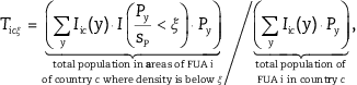 (3)
(3)
where the indicator  equals one if the population density within cell y, i.e. (Py/sP) falls short of threshold density ξ and zero otherwise. The corresponding indicator at the country level is:
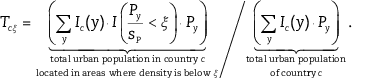 (4)
(4)
Similarly, the fraction of land with levels of population density below threshold ξ in FUA i of country c is:
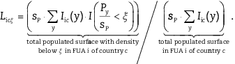 (5)
(5)
The corresponding indicator at the country level is:
 (6)
(6)
Variation of urban population density
Population density may vary substantially within a city. A measure of the variation of population density is its standard deviation. The standard deviation of population density in FUA i of country c is defined in Equation (7):
 (7)
(7)
where (Py/sP) is the population density (number of inhabitants per km2) of population cell y, PDic is the average population density of the urban area and NPic is the number of population cells that lie within the boundaries of FUA i.16
The formula in Equation (7) is used to measure the degree to which population density varies within an FUA. As explained in Chapter 2, this measure is used to detect urban areas which may display a large variation in density, while their overall density (PDic) is relatively high. An alternative, unit-free measure of density variation is the relative standard deviation of urban population density (also known as coefficient of variation), defined as:
 (8)
(8)
The standard deviation of urban population density in a country is given by:
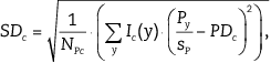 (9)
(9)
where NPc is the number of population cells that lie within the boundaries of all FUAs in country c. The rest of the terms are defined earlier in the text. The mathematical formula in Equation (9) is the standard deviation of population densities observed at all locations in the FUAs of a country from the national mean, PDc. The coefficient of variation at the country level is:
 (10)
(10)
Fragmentation
The fragmentation index (FI) measures the number of urban fabric fragments per km2 of built-up area. The mathematical formulation of the indicator is presented in Equation (11):
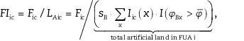 (11)
(11)
where Fic is the number of urban fabric fragments in FUA i of country c; Iic (x) equals one if the land-cover raster cell x belongs to that FUA and zero otherwise; j Bx denotes the fraction of surface in cell x that is covered by buildings or other structures; 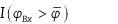 equals one if j Bx exceeds a threshold value and zero otherwise; and sB is the surface occupied by each cell in the land cover raster, which is approximately equal to 0.00146 km2 (» 38.2185 m × 38.2185 m). The variable LAic is the total surface occupied by urban fabric fragments in the FUA.17
To calculate LAic, GIS software iterates across all cells in the land cover raster, focusing on those that fall within the boundaries of the
FUA of interest. The algorithm then checks whether cell x belongs to a fragment, i.e. whether the fraction of its footprint occupied by artificial areas is at least . In this report, the threshold value was set to 0.5. This means that the indicator is given the value one whenever 50% or more of the surface of cell x is artificial, and the value of zero otherwise. The sum in the denominator of Equation (11) is the number of land-cover cells
that belong to urban fragments in urban area i. In the right panel of Figure 3.A.3, this is the number of coloured cells that results from applying the  filter to drop all cells that lie within the FUA but are not sufficiently covered by buildings or other structures. Multiplying
that number with sB yields the total artificial area within the FUA. This is the amount of land occupied by the coloured cells in the right panel of Figure 3.A.3. Constructing distinct fragments in order to obtain the numerator of Equation (11) out of the artificial land cells requires
the use of specific algorithms.18
filter to drop all cells that lie within the FUA but are not sufficiently covered by buildings or other structures. Multiplying
that number with sB yields the total artificial area within the FUA. This is the amount of land occupied by the coloured cells in the right panel of Figure 3.A.3. Constructing distinct fragments in order to obtain the numerator of Equation (11) out of the artificial land cells requires
the use of specific algorithms.18
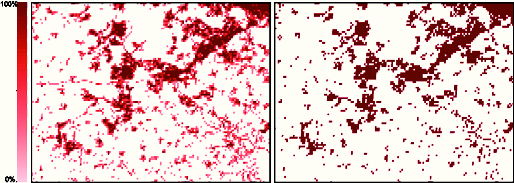
Note: Left panel: land cover map of building coverage values (j Bx). Right panel: artificial area map with red colour representing cells where building coverage exceeds 50%.
At the country level, the fragmentation index is obtained by dividing the total number of fragments identified in all functional urban areas of country c by the total amount of artificial land in the same areas. The mathematical formulation for fragmentation at the country level is:
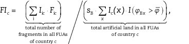 (12)
(12)
where Ic (x) equals one if the land cover raster cell x belongs to any functional urban area of country c and zero otherwise, and Iic equals one if FUA i belongs to country c and zero otherwise. The mathematical formula in Equation (12) is the expected number of urban fabric fragments per km2 in a randomly selected urban location of a country. That is equivalent to the average fragmentation observed had all FUAs of country c been concatenated in a single urban area.
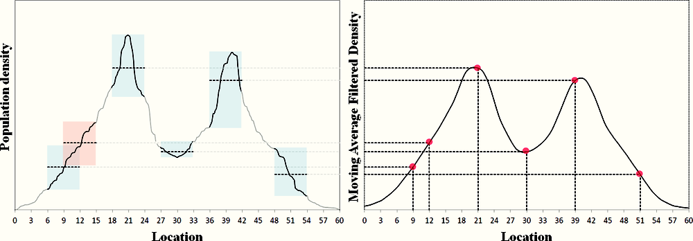
Note: The figure illustrates the process of obtaining moving average filtered densities at six different locations (9, 12, 21, 30, 39 and 51). Left panel: The width of the highlighted rectangular areas represents the bandwidth at which the moving average filter applies, i.e. 3 km towards each direction. The height of the highlighted areas represents the range of population density values within the smoothing area. The dashed lines represent the moving average population density obtained within the three kilometer bandwidth. Right panel: the values obtained from the smoothing process.
Polycentricity
Population density may peak at several locations within an FUA. In this report, urban centres are defined as areas bigger than 5 km2 where population density is substantially higher than the one observed in their surroundings. The process of extracting urban centres from their surroundings is now described in detail.
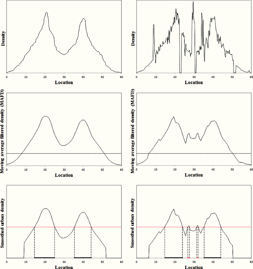
Note: Upper panels: population density across urban space. Middle panels: smoothed population density derived after applying a moving average filter. Lower panels: identification of urban centres. Left panels: a city with lower variation of local density. Right panels: a city with larger variation of population density.
First, a moving-average filter is used to smooth the density of each cell y in the population raster. The filtered density is:
 (13)
(13)
where I (y, y', d) equals one if cells y and y' fall within the same FUA and the distance between their centres is smaller than d, and zero otherwise.19 In this study, d is set at 3 km. Figure 3.A.4 provides a detailed illustration of the extraction of moving average filtered densities from the observed population densities.
The filtering process facilitates substantially the extraction of urban centres by smoothing out extremely high or low population density values. Such values may be the result of measurement errors, spatially refined regulatory mechanisms or other idiosyncratic characteristics that vary widely across very small areas. Figure 3.A.5 displays the moving average filtered densities (middle panels) for cities with low (left panels) and high (right panels) local variation of density. In both cases, the proposed filter is shown to be effective in deriving a city-wide picture of population allocation that is free of local specificities.
All cells with filtered population density below a threshold (J) are considered as rural and are therefore removed. Following OECD (2011), the threshold is set to 150 inhabitants per km2. This population density threshold is represented by the horizontal line in the middle panels of Figure 3.A.3. The outcome of removing rural areas is the smoothed population density displayed by the curves in the lower panels of Figure 3.A.5. The average smoothed density, Si, is then represented by the horizontal line in those panels. Mathematically, this can be represented by the following fraction:
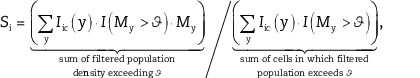 (14)
(14)
where My is the filtered population density, and 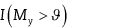 equals one if the filtered population density exceeds threshold ϑ and zero otherwise.
The set of cells in which filtered population exceeds the average smoothed density given by Equation (14) compose patches similar to those constructed out of land cover cells for built areas (see Figure 3.A.3). Any patch of population cells with total surface over 5 km2 is considered to be an urban centre. In the two dimensional illustration of Figure 3.A.5, both cities turn out to have two urban centres. The city displayed on the left yields two patches of high population density, whose footprints are projected on the horizontal axis. Since both footprints occupy a considerable amount of surface, both patches qualify to be considered as urban centres. The city displayed at the right yields four candidate urban centres; however, only two of them occupy enough space (over 5 km2) to be considered as urban centres.
The average number of urban centres in an OECD country is given by the ratio of the total number of centres identified in all functional urban areas of the country divided by the number of these urban areas. This is equivalent to the total number of urban centres expected in a randomly selected urban area of the country.
Decentralisation
Decentralisation shows the share of urban population residing outside of the urban centres of an FUA. The formula used to compute decentralisation for FUA i in country c is the one presented in Equation (15):
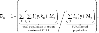 (15)
(15)
where the indicator I (y, kic) equals one if the population raster cell y belongs to urban centre k of FUA i in country c and zero otherwise. The rest of the terms are already defined in Equations (1) and (14). The decentralisation indicator is based on the use of a relative threshold density. The reason for this is that the filtered density in every cell y that belongs to an urban centre, My, will by definition exceed the city’s average smoothed density, as defined in Equation (14). Therefore, the decentralisation indicator can obtain high (low) values even in an FUA where population density is high (low) everywhere.
At the country level, decentralisation is computed according to the formula shown in Equation (16):
 (16)
(16)
where I (y, kc) equals one if the population raster cell y belongs to the urban centre k of any FUA in country c and zero otherwise. The rest of the terms are already defined in Equations (2) and (14).
Reference
OECD (2011), “Distribution of population and regional typology”, in OECD Regions at a Glance 2011, OECD Publishing, Paris, https://doi.org/10.1787/reg_glance-2011-7-en.
This Appendix presents an overview of the current situation of urban sprawl and its evolution over time for each of the 29 OECD countries considered in the study. The analysis draws on the seven indicators of urban sprawl developed earlier in this chapter. For each country, the Appendix presents: i) a box with basic statistical information and the values of urban sprawl indicators in 2014; ii) a radar chart comparing the country’s score in the urban sprawl indicators of 2014 with the average of the 29 countries included in the analysis for that year; iii) three graphs depicting the evolution of different urban sprawl indicators from 1990 until 2014; and iv) a brief discussion of the main findings from the analysis of the indicators.
The radar charts presented in panels a of Figures 3.B.1 to 3.B.29 position each country’s score in five sprawl indicators – inverse of average population density, coefficient of variation of population density within urban areas (dispersity), fragmentation of urban fabric, number of peak-density areas (polycentricity), and decentralisation of urban population – vis-à-vis the respective cross-country average in 2014. The average of the 29 countries included in the analysis is often referred to as the OECD average. The radar charts are constructed upon five axes, with each axis representing:

where xc is the average value of indicator x for all urban areas in country c, and 
is the (unweighted) OECD average. The five axes range from the minimum to the maximum value of rx, with the maximum values
denoted on the axes. The value of  for each indicator is represented by a red dot. The red dots are connected with red dashed lines, forming a pentagon that
illustrates the 29-country average for the five indicators.
for each indicator is represented by a red dot. The red dots are connected with red dashed lines, forming a pentagon that
illustrates the 29-country average for the five indicators.
The evolution of urban sprawl indicators over the period 1990-2014 is shown in panels b to d of Figures 3.B.1 to 3.B.29. The intertemporal evolution of the five indicators presented in the radar charts is presented in panels b. Instead of changes over time being shown in absolute terms, as in 3.4, they are expressed here in percentage changes. Therefore, the red dot which denotes the total percentage change in the period 1990-2014, is usually different from the sum of the individual changes (1990-2000 and 2000-14). The graphs presented in panels c and d show the intertemporal evolution of urban sprawl indicators based on absolute thresholds of population density. These indicators correspond to the percentage of populated urban areas with density levels below 1 500, 2 500 and 3 500 inhabitants per km2 and the percentage of FUA population residing in these areas.
The data sources used to produce these graphs are the ones presented in 3.3, i.e. land-cover data are provided by the Global Human Settlement (GHS) built-up area dataset (Pesaresi et al., 2015), population data by the GHS population grid (European Commission, Joint Research Centre (JRC) and Columbia University, Center for International Earth Science Information Network – CIESIN, 2015) and FUA delimitations by OECD (2012). Data on land area and population at the national level, presented in the top of the boxes for each country are provided by the World Bank (2017).
Australia

Notes: Thres. 1 denotes a population density of 1 500 inhabitants/km2, Thres. 2 a population density of 2 500 inhabitants/km2 and Thres. 3 a population density of 3 500 inhabitants/km2.
Source: Own calculations, based on GHS built-area data (Pesaresi et al., 2015), GHS population data (European Commission, Joint Research Centre (JRC) and Columbia University, Center for International Earth Science Information Network – CIESIN, 2015) and FUA delimitations (OECD, 2012).
The basic sprawl indicators of Australian urban areas are currently close to the OECD average, as shown in panel a. An exception is the polycentricity index which is 40% higher than the OECD average.
Panel b, which shows the evolution of indicators, reveals that Australian cities have undergone a densification process during the period 1990-2014. That process was especially manifested in the period from 2000 onwards: the urban areas of the country in 2014 were, on average, 16% denser than in 2000. This reveals that the footprint of urban areas has grown substantially slower than the urban population.
A similar trend is revealed by the changes occurring in the entire distribution of population density across urban space. During the period 1990-2014, the percentage of urban land with population density in the range of 150-1 500 inhabitants/km2 has steadily decreased from 59% to below 50%. That change was accompanied by a substantial increase in the percentage of urban land with density between 1 500 and 2 500 inhabitants/km2 as shown in panel c. The changes in the allocation of urban land are coupled with a similar change in the allocation of population across areas of different density levels, as shown in panel d.
At the same time, panel b suggests that there are signs that centralisation processes have been at play, as the changes in the decentralisation index have been negative for the two sub-periods of study. The evolution of the fragmentation index reveals that Australian urban areas have become slightly more contiguous in the period 2000-14, reversing a modest trend to the opposite direction in the previous period.
Austria
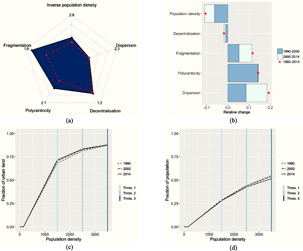
Notes: Thres. 1 denotes a population density of 1 500 inhabitants/km2, Thres. 2 a population density of 2 500 inhabitants/km2 and Thres. 3 a population density of 3 500 inhabitants/km2.
Source: Own calculations, based on GHS built-area data (Pesaresi et al., 2015), GHS population data (European Commission, Joint Research Centre (JRC) and Columbia University, Center for International Earth Science Information Network – CIESIN, 2015) and FUA delimitations (OECD, 2012).
Austrian cities are relatively sprawled, as manifested in all indicators used in this study. Austrian urban areas are approximately 40% more fragmented and polycentric than the average of the countries included in the analysis, as shown in panel a. Their population density also lies below the OECD average.
Urban sprawl has significantly increased since 1990. Average population density in Austrian cities has decreased by around 11% between 1990 and 2014, as shown in panel b. In the same period, the variation of population density across urban space increased by 19% and urban areas became more polycentric (14%) and fragmented (12%).
As depicted in panel c, the share of urban built surfaces hosting population densities within the three examined intervals (150-1 500, 1 500-2 500 and 2 500-3 500 inhabitants per km2) have remained relatively stable over time. A similar pattern is observed for the allocation of population across areas of different density, which is displayed in panel d.
Belgium
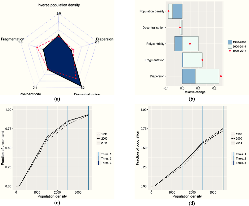
Notes: Thres. 1 denotes a population density of 1 500 inhabitants/km2, Thres. 2 a population density of 2 500 inhabitants/km2 and Thres. 3 a population density of 3 500 inhabitants/km2.
Source: Own calculations, based on GHS built-area data (Pesaresi et al., 2015), GHS population data (European Commission, Joint Research Centre (JRC) and Columbia University, Center for International Earth Science Information Network – CIESIN, 2015) and FUA delimitations (OECD, 2012).
Belgian cities are particularly decentralised, about 17% more than the OECD average, as shown in panel a. Their score in the rest of the indicators is close to the average, with one exception: Belgium’s urban areas are about 20% less fragmented. However, fragmentation has been increasing, as illustrated in panel b: between 2000 and 2014 Belgian cities have on average become 12% more fragmented. In addition, the variation of population density (dispersion) has sharply increased since 1990, by 24%. However, in 2014 dispersion still remained slightly below the OECD average.
Belgium’s urban areas have become less dense, more fragmented and more polycentric since 1990. Belgium’s urban population density has decreased by about 9% since then, while its variation has sharply increased (24%). Especially since 2000, new development has occurred in a more fragmented way and new urban centres have emerged. Fragmentation has increased by 12% and polycentricity by 10% in the period 2000-14.
Panels c and d illustrate the distribution of urban land and population to areas of low-to-moderate density levels (between 150 and 3 500 inhabitants per km2). Belgium ranks first (together with Luxembourg) among the countries included in the study in the share of urban land allocated to areas of such densities, while second in the share of population residing in them. Since 1990, the share of urban land in areas with density of 150-2 500 inhabitants per km2 has increased by about 5 percentage points, at the expense of the share of urban land in areas with density between 2 500-3 500 inhabitants per km2 (panel c). Panel d reveals a similar pattern for the share of urban population residing in areas with density between 150 and 2 500 inhabitants per km2. However, due to an important decline in the share of urban population living in areas with density of 2 500-3 500 inhabitants per km2, the percentage of urban population living in areas with low-to-moderate density is lower in 2014 than in 1990.
Canada
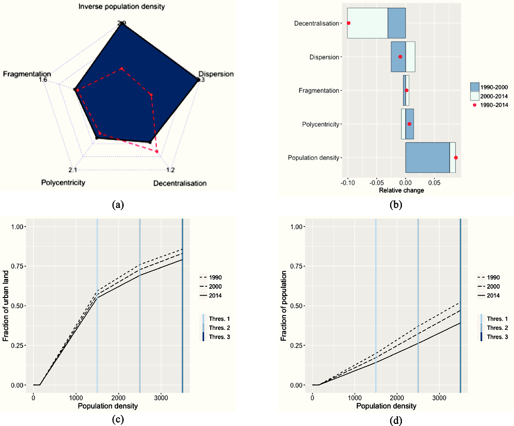
Notes: Thres. 1 denotes a population density of 1 500 inhabitants/km2, Thres. 2 a population density of 2 500 inhabitants/km2 and Thres. 3 a population density of 3 500 inhabitants/km2.
Source: Own calculations, based on GHS built-area data (Pesaresi et al., 2015), GHS population data (European Commission, Joint Research Centre (JRC) and Columbia University, Center for International Earth Science Information Network – CIESIN, 2015) and FUA delimitations (OECD, 2012).
Canada is the country with the lowest urban population density, approximately one third of the OECD average (see panel a). Furthermore, urban population density exhibits the highest variation (dispersion) in the study, about 2.3 times the OECD average.
Population density in Canadian urban areas has significantly increased between 1990 and 2014, recording a total change of 9% (panel b). However, the largest part of this reduction occurred before 2000; population density has only slightly increased since then. In contrast, centralisation forces have been rather strong since 2000: decentralisation has diminished by about 7% in the period 2000-14. In 2014, 27% of FUA population in Canada was residing outside peak-density areas considered as centres, which is below the OECD average.
The changes observed in the distribution of population density across urban space, shown in panel c, reflect the trend of increasing population density. During the period 1990-2014, the percentage of urban land with population density in the range of 150-3 500 inhabitants/km2 has steadily decreased. This reduction is especially pronounced in density levels above 1 500 inhabitants/km2. The evolution of the allocation of urban land aligns with the evolution of the allocation of population across areas of different density levels, as shown in panel d.
Chile

Notes: Thres. 1 denotes a population density of 1 500 inhabitants/km2, Thres. 2 a population density of 2 500 inhabitants/km2 and Thres. 3 a population density of 3 500 inhabitants/km2.
Source: Own calculations, based on GHS built-area data (Pesaresi et al., 2015), GHS population data (European Commission, Joint Research Centre (JRC) and Columbia University, Center for International Earth Science Information Network – CIESIN, 2015) and FUA delimitations (OECD, 2012).
Chilean urban areas are very centralised and dense. They are characterised by high population density that displays little variation (dispersion) within them, and in 2014, 78% of the urban population was residing in areas identified as urban centres (panel a). However, the country's urban areas are about 40% more fragmented than the average country included in the study.
Panel b reveals that average urban population density has increased since 1990 by about 7%, with that change mainly occurring after 2000. Variation of density has also largely decreased: since 2000, it has been reduced by 17%. At the same time, polycentricity has increased by 25% between 1990 and 2000 and has remained stable since then. Chilean urban areas have also become more fragmented, especially in the period following 2000. Overall, it seems that densification has been accompanied by higher fragmentation of urban areas.
As shown in panels c and d, the allocation of land and population to different density levels has remained rather stable during the examined period: areas with density over 3 500 inhabitants per km2 occupy more than 41% of the urban built environment and accommodate 85% of the urban population.
Czech Republic
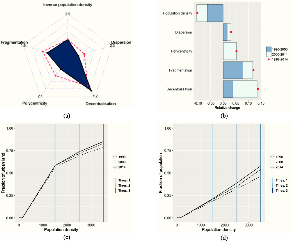
Notes: Thres. 1 denotes a population density of 1 500 inhabitants/km2, Thres. 2 a population density of 2 500 inhabitants/km2 and Thres. 3 a population density of 3 500 inhabitants/km2.
Source: Own calculations, based on GHS built-area data (Pesaresi et al., 2015), GHS population data (European Commission, Joint Research Centre (JRC) and Columbia University, Center for International Earth Science Information Network – CIESIN, 2015) and FUA delimitations (OECD, 2012).
Czech cities are generally less sprawled than the OECD average.
With the exception of decentralisation, Czech Republic lies at the OECD average or below it in all sprawl indicators (panel a). For example, polycentricity in Czech cities is about 1/3 below the OECD average. The decentralisation index is approximately 10% higher than in the average country.
The trends depicted in panel b reveal, however, that Czech cities have been sprawling since 1990. Average population density has decreased by 10%, while fragmentation and decentralisation have increased by 12% and 14% respectively. Decentralisation processes have been more pronounced in the period after 2000, accompanied by an increase in polycentricity. Despite the emergence of more urban centres, a greater number of inhabitants have decided to move outside of them.
The allocation of urban land and population over different density levels, shown in panels c and d, reflects the decrease in population density. Between 1990 and 2014, the fraction of both urban surface and population exposed to very low density levels (150-1 500 inhabitants per km2) increased by roughly two percentage points.
Denmark
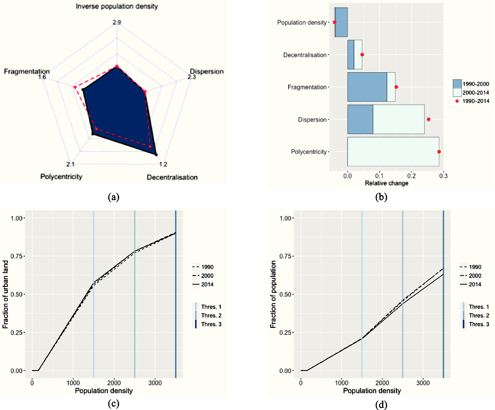
Notes: Thres. 1 denotes a population density of 1 500 inhabitants/km2, Thres. 2 a population density of 2 500 inhabitants/km2 and Thres. 3 a population density of 3 500 inhabitants/km2.
Source: Own calculations, based on GHS built-area data (Pesaresi et al., 2015), GHS population data (European Commission, Joint Research Centre (JRC) and Columbia University, Center for International Earth Science Information Network – CIESIN, 2015) and FUA delimitations (OECD, 2012).
Urban sprawl in Denmark stands relatively close to the OECD average (panel a). Danish urban areas are only slightly more fragmented and somewhat less polycentric and decentralised than cities in the average country.
Panel b shows, however, that Danish cities have sprawled significantly since 1990. They have become 15% more fragmented and the variation (dispersion) of population density within them has increased by 25%. Unlike fragmentation whose increase seems to have slowed down from 2000 onwards, the increase of the variation of density has stepped up. The most prominent indicator change in the period 2000-14 is, however, the increase of polycentricity by 28%. Average population density decreased between 1990 and 2000 but this fall has been halted after 2000.
As depicted in panel c, the share of urban surfaces hosting population densities within the three examined intervals (150-1 500, 1 500-2 500 and 2 500-3 500 inhabitants per km2) have remained relatively stable over time. A similar pattern is observed for the allocation of population across areas with densities between 150-2 500 inhabitants per km2, which is displayed in panel d. The fraction of the population residing in areas with densities between 1 500 and 3 500 inhabitants per km2 decreased slightly, by 4 percentage points.
Finland
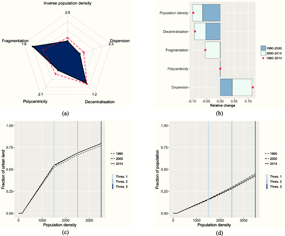
Notes: Thres. 1 denotes a population density of 1 500 inhabitants/km2, Thres. 2 a population density of 2 500 inhabitants/km2 and Thres. 3 a population density of 3 500 inhabitants/km2.
Source: Own calculations, based on GHS built-area data (Pesaresi et al., 2015), GHS population data (European Commission, Joint Research Centre (JRC) and Columbia University, Center for International Earth Science Information Network – CIESIN, 2015) and FUA delimitations (OECD, 2012).
Finnish urban areas are less sprawled than the OECD average. As shown in panel a, they are relatively dense and the variation of urban population density is relatively low. Polycentricity and decentralisation in Finland’s cities are also below the cross-country average. The only sprawl dimension along which Finnish urban areas rank higher than the average is fragmentation, by 34%.
Urban sprawl dimensions have evolved in different ways over time (panel b). Since 1990, cities have become about 10% less dense and the variation of density within them has increased by 12%. At the same time, centralisation processes have been into play, leading to a 9% reduction in the decentralisation index. Since 2000, Finnish cities have also become 5% less fragmented.
Both the distribution of urban land and the distribution of population, shown in panels c and d, remained relatively stable over time. The panels reveal a slight increase in the share of urban land and population corresponding to areas with a density between 150 to 3 500 inhabitants per km2 between 1990 and 2000, followed by a slight decrease between 2000 and 2014.
France

Notes: Thres. 1 denotes a population density of 1 500 inhabitants/km2, Thres. 2 a population density of 2 500 inhabitants/km2 and Thres. 3 a population density of 3 500 inhabitants/km2.
Source: Own calculations, based on GHS built-area data (Pesaresi et al., 2015), GHS population data (European Commission, Joint Research Centre (JRC) and Columbia University, Center for International Earth Science Information Network – CIESIN, 2015) and FUA delimitations (OECD, 2012).
French cities are very close to the cross-country average on all five dimensions of urban sprawl, as shown in panel a.
Panel b shows, however, that French urban areas have noticeably sprawled since 1990. This is manifested in the evolution of all indicators, but the greatest changes (in percentage terms) are observed in population density and polycentricity. French cities have become 12% less dense and 17% more polycentric than they were in 1990. The decrease in population density has been coupled with a 9% increase in fragmentation, which indicates that the urban areas have expanded in a discontinuous way.
Sprawling patterns in France are also revealed by the evolution of the allocation of urban land and population to areas with relatively low density. The distribution of urban land over different urban population density levels, shown in panel c, displays an increase in the portion of urban built areas hosting density levels between 150 and 3 500 inhabitants per km2: from 84% in 1990, the share increased to 88% in 2014. Cumulatively, the share of urban population residing in areas with density levels between 150 and 3 500 inhabitants per km2 (panel d) increased by 6 percentage points: from 48% in 1990 to 54% in 2014.
Germany
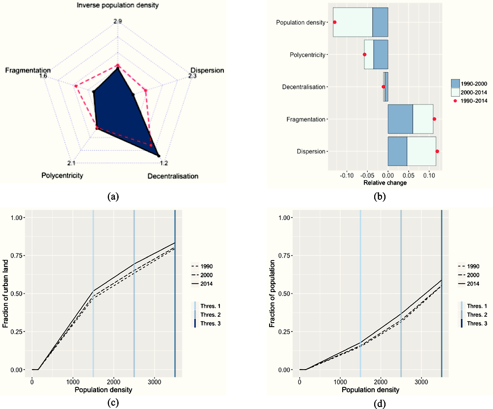
Notes: Thres. 1 denotes a population density of 1 500 inhabitants/km2, Thres. 2 a population density of 2 500 inhabitants/km2 and Thres. 3 a population density of 3 500 inhabitants/km2.
Source: Own calculations, based on GHS built-area data (Pesaresi et al., 2015), GHS population data (European Commission, Joint Research Centre (JRC) and Columbia University, Center for International Earth Science Information Network – CIESIN, 2015) and FUA delimitations (OECD, 2012).
Compared to the OECD average in 2014, German urban areas are more decentralised and contiguous (panel a). Urban population density is slightly above the average and displays a relatively low variation.
Since 1990, Germany has followed a sprawling process (panel b). Between 1990 and 2014, urban population density decreased by about 13%, while its variation (dispersion) increased by 12%. German urban areas have also become 12% more fragmented than they were in 1990.
As shown in panel c, the decrease in population density between 1990 and 2014 has been accompanied by an increase of five percentage points (47% to 52%) in the share of urban land hosting very low population density levels (150-1 500 inhabitants per km2). The corresponding increase in the share of population, shown in panel d, is three percentage points: from 15% to 18%.
Greece

Notes: Thres. 1 denotes a population density of 1 500 inhabitants/km2, Thres. 2 a population density of 2 500 inhabitants/km2 and Thres. 3 a population density of 3 500 inhabitants/km2.
Source: Own calculations, based on GHS built-area data (Pesaresi et al., 2015), GHS population data (European Commission, Joint Research Centre (JRC) and Columbia University, Center for International Earth Science Information Network – CIESIN, 2015) and FUA delimitations (OECD, 2012).
Greek urban areas are among the most compact of those included in the study (panel a). Greece ranks fourth in average urban population density and contains exclusively monocentric urban areas that display the minimum decentralisation recorded in the study. Fragmentation and variation of urban population density (dispersion) are very close to the OECD average values.
As shown in panel b, Greek urban areas have sprawled since 2000. Average urban population density has decreased by about 5% during that period, while its variation has slightly increased. Fragmentation has been rising since 1990, exhibiting an increase of about 11% in the entire period of study.
The distribution of the urban area and the population over different population density levels is shown in panel c and panel d respectively. The percentage of the urban area exposed to densities between 150 and 3 500 people/km2 increased in both periods of the study, whereas the distribution of the population at those density levels remained rather stable.
Hungary

Notes: Thres. 1 denotes a population density of 1 500 inhabitants/km2, Thres. 2 a population density of 2 500 inhabitants/km2 and Thres. 3 a population density of 3 500 inhabitants/km2.
Source: Own calculations, based on GHS built-area data (Pesaresi et al., 2015), GHS population data (European Commission, Joint Research Centre (JRC) and Columbia University, Center for International Earth Science Information Network – CIESIN, 2015) and FUA delimitations (OECD, 2012).
Hungarian cities are close to the OECD average in most urban sprawl indicators, with the exception of decentralisation and polycentricity. They are 33% less polycentric and 7% more decentralised than the average country, as shown in panel a.
Panel b shows that while Hungarian cities have become less dense and more fragmented since 1990, they have also become less polycentric and decentralised. Urban population density fell by 24% in the examined period, with the largest part of this change occurring from 2000 onwards. Since that year, the number of urban centres has also decreased by 32%, the largest decrease in the polycentricity index recorded in this study. On the other hand, the variation of urban population density and fragmentation have significantly increased since 1990, by about 29%.
One of the drivers of the reduction of average population density is the increase in the share of urban surfaces hosting very low densities (150-1 500 inhabitants per km2) by 9 percentage points (panel c). In contrast, the share of urban surface corresponding to population densities between 2 500 and 3 500 inhabitants per km2 was reduced in the examined period. This has been accompanied by a decline in the share of population residing in areas with such densities (panel d). The share of urban population living in areas with density below 3 500 inhabitants per km2 was lower in 2014 than in 1990.
Ireland
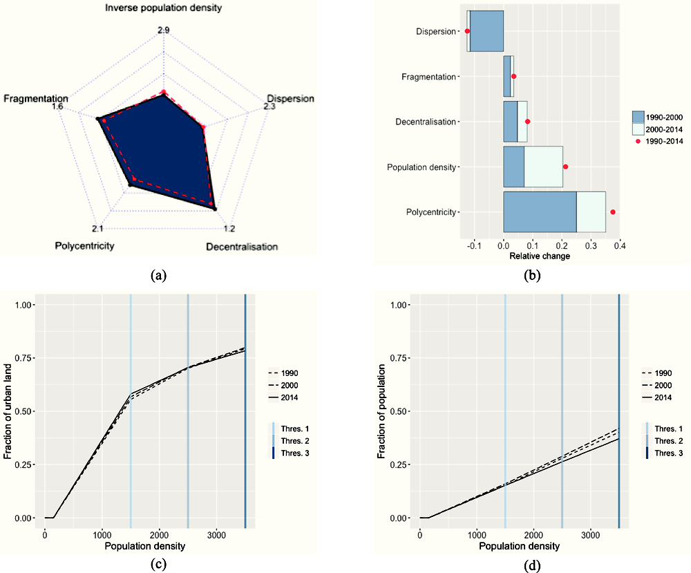
Notes: Thres. 1 denotes a population density of 1 500 inhabitants/km2, Thres. 2 a population density of 2 500 inhabitants/km2 and Thres. 3 a population density of 3 500 inhabitants/km2.
Source: Own calculations, based on GHS built-area data (Pesaresi et al., 2015), GHS population data (European Commission, Joint Research Centre (JRC) and Columbia University, Center for International Earth Science Information Network – CIESIN, 2015) and FUA delimitations (OECD, 2012).
Irish urban areas were, in 2014, close to the OECD average in all five sprawl dimensions shown in panel a.
The trends depicted in panel b, however, reveal a less typical pattern. Ireland experienced a 21% increase in population density between 1990 and 2014, but new development was realised in a polycentric and decentralised fashion: urban areas became 38% more polycentric and 8% more decentralised. This is the largest increase in the polycentricity index recorded in the study.
Despite the large increase in average population density, the share of areas hosting densities between 150 and 3 500 inhabitants per km2 remained rather stable (panel c). At the same time, the share of population living in areas of such densities has slightly decreased (panel d). This is mainly driven by a small reduction in the share of population residing in densities between 1 500 and 2 500 inhabitants per km2.
Italy
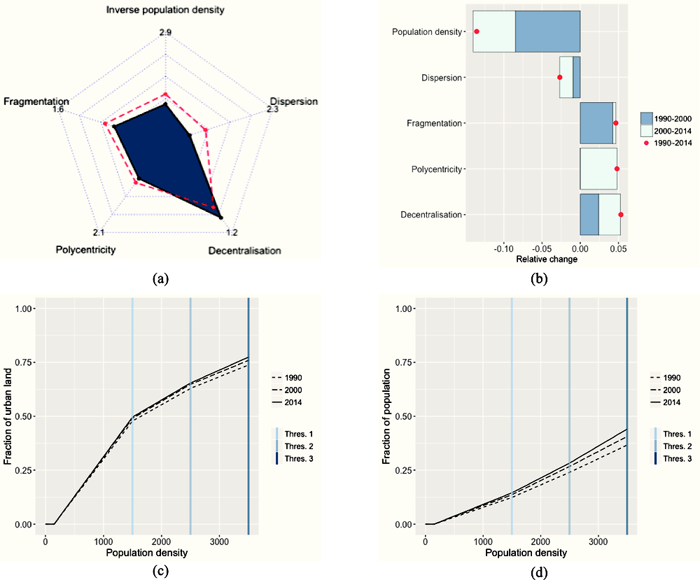
Notes: Thres. 1 denotes a population density of 1 500 inhabitants/km2, Thres. 2 a population density of 2 500 inhabitants/km2 and Thres. 3 a population density of 3 500 inhabitants/km2.
Source: Own calculations, based on GHS built-area data (Pesaresi et al., 2015), GHS population data (European Commission, Joint Research Centre (JRC) and Columbia University, Center for International Earth Science Information Network – CIESIN, 2015) and FUA delimitations (OECD, 2012).
Urban sprawl in Italy is below the OECD average with respect to multiple dimensions. The only exception is decentralisation, where Italian cities lie considerably above the OECD average (panel a).
Italy’s urban population density has decreased by 14% since 1990, as shown in panel b. Despite that decline, Italy’s average urban population density was still above the OECD average, by 30%, in 2014. In addition to being less dense, new development was realised in a fragmented and decentralised way, with both indicators increasing by 5% between 1990 and 2014.
Panel c reveals that the large reduction of average population density has not been accompanied by an equally pronounced increase in the share of urban land hosting surfaces with density between 150 and 3 500 inhabitants/km2. While that share has only grown by 3 percentage points, the share of urban population residing in these areas has increased from 37% in 1990 to 44% in 2014 (panel d).
Japan
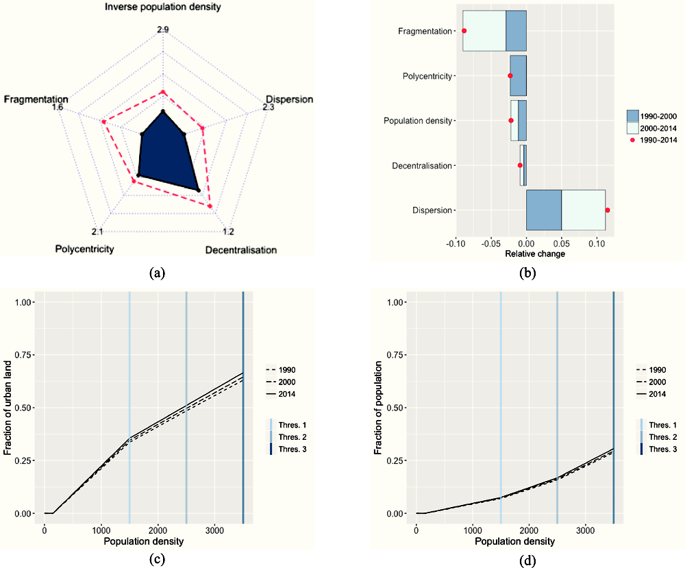
Notes: Thres. 1 denotes a population density of 1 500 inhabitants/km2, Thres. 2 a population density of 2 500 inhabitants/km2 and Thres. 3 a population density of 3 500 inhabitants/km2.
Source: Own calculations, based on GHS built-area data (Pesaresi et al., 2015), GHS population data (European Commission, Joint Research Centre (JRC) and Columbia University, Center for International Earth Science Information Network – CIESIN, 2015) and FUA delimitations (OECD, 2012).
Japanese cities are compact, dense and centralised. They score relatively low in all dimensions of urban sprawl, as shown in panel a. Urban population density lies far above the OECD average and displays the lowest variation (dispersion) across the OECD countries. Japanese urban areas are the most contiguous, with only 4.9 fragments per km2 of built area.
The evolution of these sprawl indicators over time is displayed in panel b. Indicators changed only modestly between 1990 and 2014, with two exceptions. Despite variation of population density being relatively low in 2014, it has increased by approximately 12% since 1990. On the other hand, urban areas in Japan became substantially more contiguous (by about 9%) in the examined period, with the largest part of this change taking place from 2000 onwards.
As can be seen from panel c, the share of urban developed surfaces hosting population densities within the three proposed intervals (150-1 500, 1 500-2 500 and 2 500-3 500 inhabitants per km2) has remained relatively stable over time. A similar pattern is observed for the allocation of population across areas of different density, which is displayed in panel d.
Korea
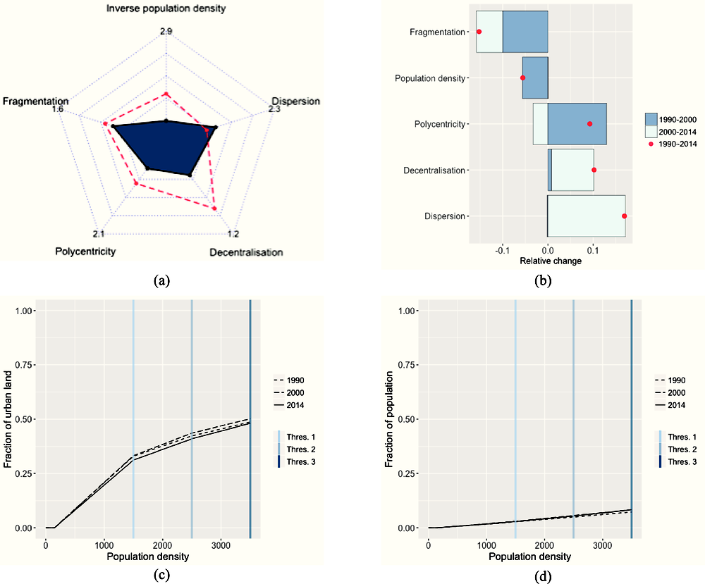
Notes: Thres. 1 denotes a population density of 1 500 inhabitants/km2, Thres. 2 a population density of 2 500 inhabitants/km2 and Thres. 3 a population density of 3 500 inhabitants/km2.
Source: Own calculations, based on GHS built-area data (Pesaresi et al., 2015), GHS population data (European Commission, Joint Research Centre (JRC) and Columbia University, Center for International Earth Science Information Network – CIESIN, 2015) and FUA delimitations (OECD, 2012).
Korean urban areas are the densest among the 29 OECD countries considered in the study: their population density is 82% higher than the OECD average. Urban fabric in the country is relatively contiguous and residential locations particularly centralised. As shown in panel a, Korean cities score relatively low in all indicators except for dispersion, which lies 17% above the OECD average.
Korean urban areas used to be even denser and centralised in the past (panel b), as average population density decreased by 6% between 1990 and 2000 and decentralisation increased by 10% between 2000 and 2014. Since 2000, there has also been a significant (17%) increase in the variation (dispersion) of urban population density. On the other hand, urban fabric in Korea has become considerably (15%) more contiguous than it was in 1990.
The dominant urban development pattern in Korea is reflected in panel c and panel d, which show the distribution of the urban built surface and urban population across three different segments of population density. Among the examined countries, cities in Korea are characterised by the lowest share of urban land hosting residential areas of density between 150 and 3 500 inhabitants per km2 (48%) and the lowest percentage of population residing in them (8%). That pattern is very similar when areas of very low density (between 150-1 500 inhabitants per km2) are considered instead. The evolution of the two distributions has remained relatively stable over time.
Luxembourg
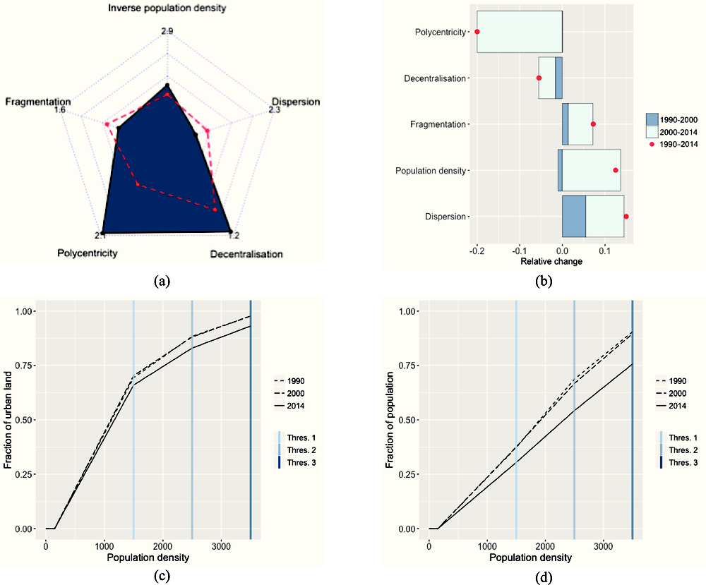
Notes: Thres. 1 denotes a population density of 1 500 inhabitants/km2, Thres. 2 a population density of 2 500 inhabitants/km2 and Thres. 3 a population density of 3 500 inhabitants/km2.
Source: Own calculations, based on GHS built-area data (Pesaresi et al., 2015), GHS population data (European Commission, Joint Research Centre (JRC) and Columbia University, Center for International Earth Science Information Network – CIESIN, 2015) and FUA delimitations (OECD, 2012).
Luxembourg comprises only one functional urban area that occupies a large part (82%) of the country’s surface. As shown in panel a, that urban area is relatively contiguous and its average population density lies 28% lower than the OECD average. The sole FUA of the country is more decentralised (17%) and contains twice as many urban centres as the average OECD urban area does. The value of the polycentricity indicator is the largest recorded in the study.
Luxembourg’s urban area has become significantly denser, less polycentric and more centralised since 2000, as shown in panel b. Population density has increased by approximately 15%, polycentricity has declined by 20% and decentralisation by 4%. However, new development has occurred in a rather fragmented way, as indicated by the 6% increase in fragmentation since 2000. Since 1990, the variation of urban population density (dispersion) in Luxembourg has increased by 15%. Even then, however, variation remained low compared to other countries included in the study.
Among the OECD countries included in the analysis, Luxembourg has the highest share of urban land and urban population allocated to areas of low to moderate density, i.e. between 150 and 3 500 inhabitants per km2. As shown in panel c, the share of urban built surfaces hosting residential areas of densities between 150 and 3 500 inhabitants per km2 decreased by about 5 percentage points between 1990 and 2014. That change was accompanied by a sharp reduction in the percentage of population residing in such density levels by about 15 percentage points, as panel d suggests. Most of this reduction is due to the decline of the share of population residing in areas between 1 500 and 2 500 inhabitants per km2.
Mexico
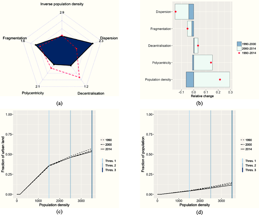
Notes: Thres. 1 denotes a population density of 1 500 inhabitants/km2, Thres. 2 a population density of 2 500 inhabitants/km2 and Thres. 3 a population density of 3 500 inhabitants/km2.
Source: Own calculations, based on GHS built-area data (Pesaresi et al., 2015), GHS population data (European Commission, Joint Research Centre (JRC) and Columbia University, Center for International Earth Science Information Network – CIESIN, 2015) and FUA delimitations (OECD, 2012).
Mexican cities are more fragmented than the average of the countries included in the study, but also less polycentric and decentralised (panel a). While their population density lies close to the OECD average, it varies across urban space much more (86%) than the OECD average.
Since 2000, Mexican cities have become much denser and more polycentric, while the variation of density within them has decreased (panel b). Population density has increased by 29% and polycentricity by 15%, while the variation of population density has declined by about 11%. During the same period (2000-14), fragmentation has declined by approximately 4%.
The share of urban developed surfaces hosting residential areas of population density between 150 and 3 500 inhabitants per km2 has decreased by approximately four percentage points: from 57% in 1990 to 53% in 2014 (panel c). The largest part of this change is due to a decline in the share of urban land hosting density levels between 2 500 and 3 500 inhabitants per km2. This implies that some of these areas have densified and crossed the threshold of 3 500 inhabitants per km2 during the time period covered in the study. A similar pattern is observed with respect to the share of urban population residing in density levels between 2 500 and 3 500 inhabitants per km2 (panel d).
Netherlands
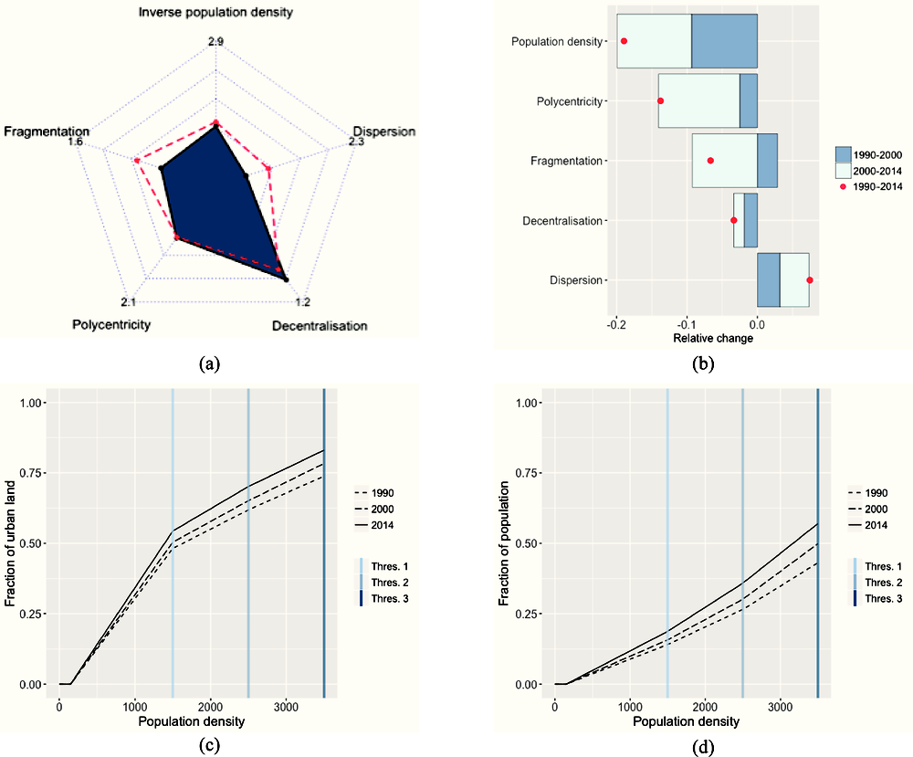
Notes: Thres. 1 denotes a population density of 1 500 inhabitants/km2, Thres. 2 a population density of 2 500 inhabitants/km2 and Thres. 3 a population density of 3 500 inhabitants/km2.
Source: Own calculations, based on GHS built-area data (Pesaresi et al., 2015), GHS population data (European Commission, Joint Research Centre (JRC) and Columbia University, Center for International Earth Science Information Network – CIESIN, 2015) and FUA delimitations (OECD, 2012).
Dutch urban areas are less fragmented, but also more decentralised than the OECD average (panel a). The variation of population density (dispersion) across urban space in the Netherlands lies far below the respective OECD average.
The Netherlands has experienced a suburbanisation process since 1990, mainly manifested in a 19% reduction of the population density (panel b). New developments seem, however, to have been constructed in a more contiguous manner; this is reflected in a 9% reduction of the fragmentation index in the period between 2000 and 2014. During the same period, the number of urban centres declined by 14%, whereas the variation of population density increased by about 4%.
The sharp decrease in population density is reflected in the changes occurred in the way urban land is allocated across different density levels (panel c). The share of urban built surface hosting residential areas of very low population density (150-1 500 inhabitants per km2) increased gradually from 48% in 1990 to 54% in 2014. The respective increase in the share of land hosting density of 1 500-2 500 and 2 500-3 500 inhabitants per km2 is substantially smaller. This suggests that new development of very low density is the main driver behind the fall of average population density in Dutch urban areas. Panel d displays the evolution of the allocation of population across the three different density segments considered in the study. The share of population living in areas of density between 150 and 3 500 inhabitants per km2 has sharply increased in the examined period, from 43% in 1990 to 57% in 2014.
Norway

Notes: Thres. 1 denotes a population density of 1 500 inhabitants/km2, Thres. 2 a population density of 2 500 inhabitants/km2 and Thres. 3 a population density of 3 500 inhabitants/km2.
Source: Own calculations, based on GHS built-area data (Pesaresi et al., 2015), GHS population data (European Commission, Joint Research Centre (JRC) and Columbia University, Center for International Earth Science Information Network – CIESIN, 2015) and FUA delimitations (OECD, 2012).
Most of the sprawl indicators values for Norwegian cities lie close to the OECD average (panel a). Urban areas in Norway are slightly more fragmented and decentralised than the OECD average while the variation of population density (dispersion) and the polycentricity index values are slightly below the average.
Among the 29 countries included in the study, Norway experienced the largest increase in population density between 1990 and 2014, as during that period Norwegian urban areas densified by 26%. During the same period, urban areas developed in a relatively more contiguous and centralised way, as fragmentation decreased by 10% and decentralisation by 5%.
As it can be seen from panel c, the share of urban built surfaces hosting population densities between 1 500 and 2 500 inhabitants per km2 decreased slightly over time. A similar, but relatively stronger, pattern is observed for the allocation of population across areas of different density, which is displayed in panel d. The share of population residing in areas of densities between 150 and 3 500 inhabitants per km2 has declined from 59% in 1990 to 52% in 2014. Most of this decline has occurred in areas of densities of 1 500-2 500 inhabitants per km2.
Poland

Notes: Thres. 1 denotes a population density of 1 500 inhabitants/km2, Thres. 2 a population density of 2 500 inhabitants/km2 and Thres. 3 a population density of 3 500 inhabitants/km2.
Source: Own calculations, based on GHS built-area data (Pesaresi et al., 2015), GHS population data (European Commission, Joint Research Centre (JRC) and Columbia University, Center for International Earth Science Information Network – CIESIN, 2015) and FUA delimitations (OECD, 2012).
Polish urban areas are denser, less polycentric and more fragmented than the OECD average (panel a). Population density displays a variation (dispersion) that is 20% lower than the OECD average.
The most prominent trend in the evolution of urban sprawl in Poland is the sharp reduction of population density between 1990 and 2014 (panel b). The latter has declined by 21%, with the largest part of this reduction occurring in the period between 2000 and 2014. The reduction of average population density was accompanied by a 7% increase in fragmentation and a 5% increase in decentralisation.
The distribution of urban land and population over different density levels, shown in panel c and panel d, reflects the decrease in average population density. Between 1990 and 2014, the share of built surfaces hosting areas of low-to-moderate population density (between 150 and 3 500 inhabitants per km2) increased by 6 percentage points: from 75% in 1990 to 81% in 2014 (panel c). During the same period, the share of population residing in areas of such densities increased from 35% to 45% (panel d). Population increased particularly in areas of low density, i.e. between 150 and 2 500 inhabitants per km2.
Portugal
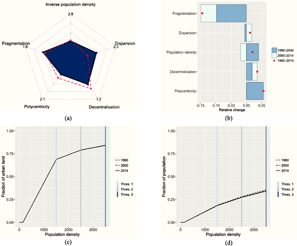
Notes: Thres. 1 denotes a population density of 1 500 inhabitants/km2, Thres. 2 a population density of 2 500 inhabitants/km2 and Thres. 3 a population density of 3 500 inhabitants/km2.
Source: Own calculations, based on GHS built-area data (Pesaresi et al., 2015), GHS population data (European Commission, Joint Research Centre (JRC) and Columbia University, Center for International Earth Science Information Network – CIESIN, 2015) and FUA delimitations (OECD, 2012).
Portuguese cities are relatively centralised and their population density lies close to the OECD average (panel a). However, population density exhibits a large variation across the urban fabric. This is reflected in the dispersion indicator that lies 40% above the OECD average. Portuguese urban areas tend to be monocentric, while the fragmentation index lies very close to the OECD average.
The evolution of urban sprawl indicator between 1990 and 2014 does not reveal major changes, with the exception of a 14% reduction in fragmentation (panel b). Furthermore, some new urban centres emerged in Portuguese urban areas between 1990 and 2000.
The fraction of urban land occupied by low density areas (150-3 500 inhabitants per km2) has remained relatively stable in the period 1990-2014, as panel c suggests. A similar trend is also observed in the evolution of the fraction of population residing in those areas, as shown in panel d.
Slovak Republic
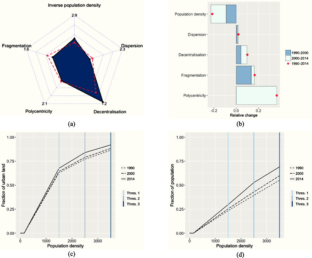
Notes: Thres. 1 denotes a population density of 1 500 inhabitants/km2, Thres. 2 a population density of 2 500 inhabitants/km2 and Thres. 3 a population density of 3 500 inhabitants/km2.
Source: Own calculations, based on GHS built-area data (Pesaresi et al., 2015), GHS population data (European Commission, Joint Research Centre (JRC) and Columbia University, Center for International Earth Science Information Network – CIESIN, 2015) and FUA delimitations (OECD, 2012).
Slovak cities are decentralised and less dense than the OECD average, but they also exhibit a lower fragmentation of the urban fabric (panel a). Per capita land consumption (inverse of population density) in Slovak Republic’s eight functional urban areas is 29% higher than the OECD average; the variation of urban population density (dispersion) is 11% lower than the corresponding OECD average.
Since 1990, Slovak urban areas have sprawled substantially. As shown in panel b, average population density has declined by 22%, while decentralisation and fragmentation have increased by 10% and 17% respectively. New urban centres have emerged between 2000 and 2014, when polycentricity increased by 36%.
The decreasing average population density has been coupled with sharp changes in the way urban surfaces and population are allocated across different population density segments. Between 1990 and 2014, the share of built surfaces hosting areas of low population density (between 150 and 3 500 inhabitants per km2) increased considerably: from 86% in 1990 to 92% in 2014 (panel c). This is the third highest value of the indicator recorded in the study for that year. The share of population residing in areas of low population density increased by 14 percentage points in the examined period: from 55% in 1990 to 69% in 2014 (panel d).
Slovenia

Notes: Thres. 1 denotes a population density of 1 500 inhabitants/km2, Thres. 2 a population density of 2 500 inhabitants/km2 and Thres. 3 a population density of 3 500 inhabitants/km2.
Source: Own calculations, based on GHS built-area data (Pesaresi et al., 2015), GHS population data (European Commission, Joint Research Centre (JRC) and Columbia University, Center for International Earth Science Information Network – CIESIN, 2015) and FUA delimitations (OECD, 2012).
Slovenia’s two functional urban areas, Ljubljana and Maribor, are relatively sprawled. They are very decentralised, fragmented and sparsely populated (panel a). The country average of fragmentation and decentralisation are the highest recorded in the study, 54% and 22% higher than the OECD average respectively. Average urban population density is also low, less than half of the average OECD country.
Evolution of sprawl over time shows, however, some slightly encouraging trends. Between 1990 and 2014, Slovenian urban areas have densified by about 16%, as shown in panel b. Cities have also become somewhat less decentralised in that period, while variation of urban population density (dispersion) has declined by about 8%.
Panel c and panel d show that the way urban built surfaces and population are distributed across different population density segments has remained relatively stable since 1990. The densification observed in the examined period has not been translated in a noticeable reduction of the share of urban land and population in areas of low-to-moderate density (between 150-3 500 inhabitants per km2).
Spain
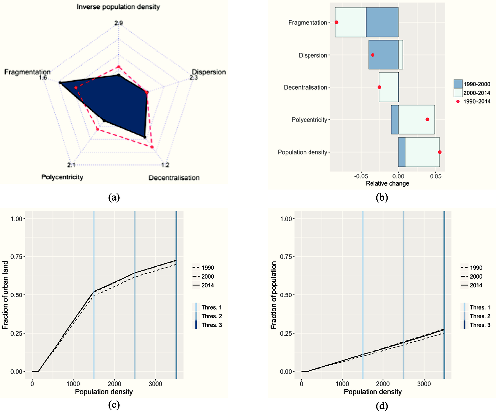
Notes: Thres. 1 denotes a population density of 1 500 inhabitants/km2, Thres. 2 a population density of 2 500 inhabitants/km2 and Thres. 3 a population density of 3 500 inhabitants/km2.
Source: Own calculations, based on GHS built-area data (Pesaresi et al., 2015), GHS population data (European Commission, Joint Research Centre (JRC) and Columbia University, Center for International Earth Science Information Network – CIESIN, 2015) and FUA delimitations (OECD, 2012).
Spanish urban areas are rather dense and centralised, have relatively fewer centres and are more fragmented than the OECD average (panel a). Land consumed per person in urban areas is 35% lower than the OECD average, while polycentricity and decentralisation are below cross-country averages by 27% and 12% respectively. On the other hand, urban fabric in Spanish cities is more fragmented than the OECD average.
Since 1990, Spanish cities have become denser, less fragmented and less decentralised (panel b). Population density has increased by 6% in the examined period, with most of this change occurring after 2000, while fragmentation has decreased by 8%. The number of urban centres has increased slightly (3%) since 2000.
The distributions of urban land and population over different density levels, shown in panels c and d, reflect that the increase in average population density between 1990 and 2014 has been accompanied by a parallel process of suburbanisation. The share of urban built surface and urban population in areas with densities of 150-3 500 inhabitants per km2 slightly increased (by 2-3 percentage points) in that period.
Sweden
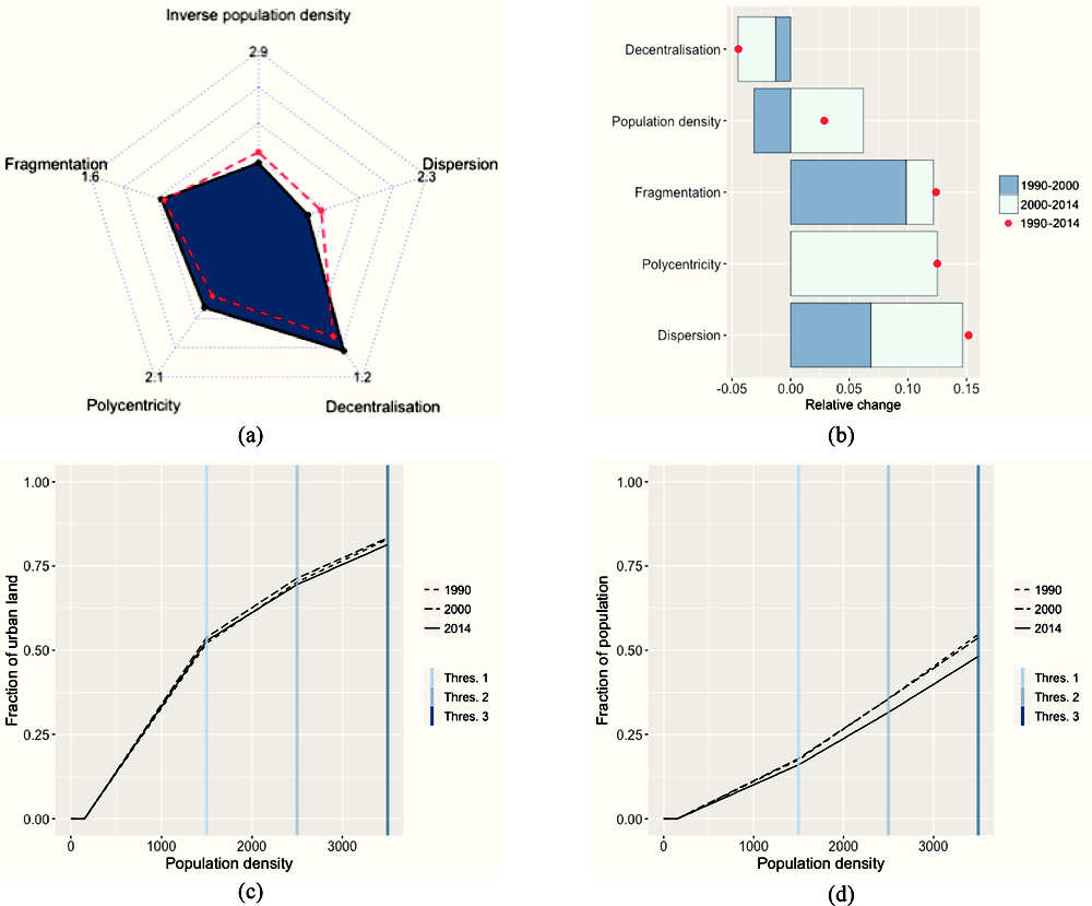
Notes: Thres. 1 denotes a population density of 1 500 inhabitants/km2, Thres. 2 a population density of 2 500 inhabitants/km2 and Thres. 3 a population density of 3 500 inhabitants/km2.
Source: Own calculations, based on GHS built-area data (Pesaresi et al., 2015), GHS population data (European Commission, Joint Research Centre (JRC) and Columbia University, Center for International Earth Science Information Network – CIESIN, 2015) and FUA delimitations (OECD, 2012).
Swedish urban areas are denser than the OECD average. They are also rather polycentric and decentralised (panel a). The variation of population density within Swedish cities (dispersion) is smaller than the OECD average.
In 2014 Swedish cities were more fragmented, centralised and polycentric than they were in 1990 (panel b). In the examined period (1990-2014), fragmentation of urban fabric and the variation of urban population density (dispersion) increased by 12% and 15% respectively. New urban centres have emerged in Swedish cities since 2000, increasing polycentricity by about 13%. On the other hand, decentralisation declined by 4% between 1990 and 2014 and population density increased by 6% between 2000 and 2014.
Panel c and panel d summarise the way urban surfaces and population are distributed across different population density segments. During the period 1990-2014, the percentage of urban population residing in areas where population density is relatively low (i.e. 150-3 500 inhabitants per km2) has decreased by 7 percentage points (panel d). The share of urban surfaces hosting residential areas of such density levels exhibit a much smaller decrease of 2 percentage points in the same period (panel c).
Switzerland

Notes: Thres. 1 denotes a population density of 1 500 inhabitants/km2, Thres. 2 a population density of 2 500 inhabitants/km2 and Thres. 3 a population density of 3 500 inhabitants/km2.
Source: Own calculations, based on GHS built-area data (Pesaresi et al., 2015), GHS population data (European Commission, Joint Research Centre (JRC) and Columbia University, Center for International Earth Science Information Network – CIESIN, 2015) and FUA delimitations (OECD, 2012).
Swiss urban areas are relatively dense and developed on a rather contiguous urban fabric (panel a). However, they are also more decentralised and polycentric than the OECD average. Fragmentation is considerably lower than the average of the countries included in the analysis, while urban population density also exhibits a variation (dispersion) which is 24% lower than the corresponding average.
The main features of the evolution of urban sprawl since 1990 are a sharp increase of population density and a small reduction of polycentricity (panel b). Population density has increased by 14% since 1990 and by 11% since 2000, while polycentricity declined by about 5% between 1990 and 2000.
The increase in average density is also reflected in the distribution of the urban area and population over different density levels, shown in panel c and d. The share of urban population residing in areas of density between 150 and 3 500 inhabitants per km2 decreased by about 7 percentage points between 1990 and 2014 (panel d). Over the same period, the share of urban surfaces hosting residential areas of density between 150 and 3 500 inhabitants per km2 decreased by approximately 4 percentage points (panel c).
United Kingdom

Notes: Thres. 1 denotes a population density of 1 500 inhabitants/km2, Thres. 2 a population density of 2 500 inhabitants/km2 and Thres. 3 a population density of 3 500 inhabitants/km2.
Source: Own calculations, based on GHS built-area data (Pesaresi et al., 2015), GHS population data (European Commission, Joint Research Centre (JRC) and Columbia University, Center for International Earth Science Information Network – CIESIN, 2015) and FUA delimitations (OECD, 2012).
The urban areas of the United Kingdom are relatively dense, compact and centralised. Urban population density is much higher than the OECD average and exhibits a rather low variation across urban space. Urban fabric is particularly contiguous, as it contains just five fragments per km2, i.e. half of the OECD average (panel a).
Since 1990, British urban areas have become much more fragmented, but also slightly denser, as shown in panel b. United Kingdom’s urban areas underwent the largest total increase in fragmentation observed in the study, with urban areas becoming 37% more fragmented. Variation of population density within urban areas (dispersion) has also increased by 11% since 1990.
As can be seen from panel c, the share of urban built surfaces hosting population densities within the three examined intervals (150-1 500, 1 500-2 500 and 2 500-3 500 inhabitants per km2) has remained relatively stable over time. The share of urban population residing in areas of such densities has declined by 3 percentage points since 1990, mainly due a reduction of the share of population living in areas of density between 1 500 and 2 500 inhabitants per km2 (panel d).
United States
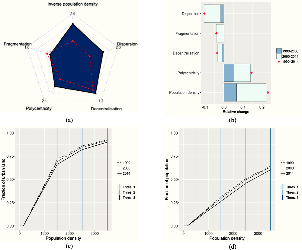
Notes: Thres. 1 denotes a population density of 1 500 inhabitants/km2, Thres. 2 a population density of 2 500 inhabitants/km2 and Thres. 3 a population density of 3 500 inhabitants/km2.
Source: Own calculations, based on GHS built-area data (Pesaresi et al., 2015), GHS population data (European Commission, Joint Research Centre (JRC) and Columbia University, Center for International Earth Science Information Network – CIESIN, 2015) and FUA delimitations (OECD, 2012).
United States’ urban areas are sparsely populated, polycentric and rather decentralised, but also less fragmented than the average of the countries included in this analysis (panel a). Population density is on average very low and varies widely across a relatively contiguous urban fabric. The country also contains the most polycentric urban areas identified in this study: Washington and New York.
Since 1990, cities of the United States have significantly densified and have become less fragmented and decentralised (panel b). Population density has increased by 23% since 1990, with most of this change taking place after 2000. At the same time, the variation of urban population density across urban space (dispersion) has declined by about 10%. Several new centres have also emerged within urban areas since 1990, leading to a 14% increase in polycentricity.
The densification process identified above is also reflected in a reduction of the share of urban land and population allocated to areas of low density. The distribution of urban land across different density levels, displayed in panel c, shows that the share of very low density areas (150-1 500 inhabitants per km2) in total urban built area decreased by about 5 percentage points between 1990 and 2014. The respective decline in the share of urban land allocated to areas of density between 150 and 3 500 inhabitants per km2 was, however, much smaller: from 92% in 1990 to 90% in 2014. At the same time, the share of population residing in those areas decreased slightly from 64% in 1990 to 60% in 2014, as panel d suggests.
References
European Commission, Joint Research Centre (JRC) and Columbia University, Center for International Earth Science Information Network – CIESIN (2015), “GHS population grid, derived from GPW4, multitemporal (1975, 1990, 2000, 2015)” (database), European Commission, Joint Research Centre (JRC), http://data.europa.eu/89h/jrc-ghsl-ghs_pop_gpw4_globe_r2015a.
OECD (2012), Redefining “Urban”: A New Way to Measure Metropolitan Areas, OECD Publishing, Paris, https://doi.org/10.1787/9789264174108-en.
Pesaresi, M. et al. (2015), “GHS built-up grid, derived from Landsat, multitemporal (1975, 1990, 2000, 2014)” (database), European Commission, Joint Research Centre (JRC), http://data.europa.eu/89h/jrc-ghsl-ghs_built_ldsmt_globe_r2015b.
World Bank (2017), World Development Indicators (database), World Bank, http://databank.worldbank.org/data/reports.aspx?source=world-development-indicators (accessed 24 November 2017).
Notes
← 1. The terms “indicator” and “metric” are used interchangeably throughout this chapter.
← 2. Non-artificial surfaces inside urban areas may include, among others, agricultural areas, forests, grasslands and water bodies.
← 3. In the terminology used by Eurostat, this translates into Local Administrative Units (LAU) level 2, formerly known as NUTS level 5. An exception is Portugal, for which commuting data are available at the LAU-1 level.
← 4. A raster map is organizes geographic information using a grid consisting of equally sized cells.
← 5. The population grid data used in the identification of urban cores have been derived from population census data at the municipality level using downscaling techniques. Such techniques provide an allocation of the municipal populations, which are usually available through census data, to higher resolution grid cells using land cover and land-use data, coupled with interpolation techniques. The latter techniques are used to distribute population in a high-resolution manner. The former are used to ensure that the spatial distribution will accord to the observed land-cover and land-use patterns. Thus, population will be allocated only to artificial and not to, for example, agricultural or forest areas. In the case of Europe, the population grid was derived by the Joint Research Centre (JRC) at 1 km2 resolution combining census data at the LAU-2 level with CORINE land cover and other data sources for land use. For all non-European countries, harmonised gridded population data from the Landscan project are used.
← 6. Formore information, see http://ghsl.jrc.ec.europa.eu/index.php.
← 7. The intermediate steps of orthorectification, georeferencing, spectral calibration and radiometric corrections that are followed between the receipt of satellite images and the production of settlement data are out of the scope of this discussion.
← 8. It should be noted that the employed datasets for human settlements can neither distinguish between different types of land use (i.e. residential, commercial, industrial etc.), nor account for vertical intensity of development, i.e. building height. Therefore, the derived grid population data will overestimate population in cells where floor space is predominantly industrial or commercial. Population density may be overestimated in areas where structural density (i.e. the floor-to-area ratio) is low and underestimated where it is high. Despite the above imperfections, the allocation of population within the grid cells of an administrative area is a valid approximation at the aggregate level.
← 9. Functional urban area boundaries have not yet been specified for Iceland, Israel, Latvia, New Zealand and Turkey, and, thus, indicator values could not be computed for these countries. Global Human Settlement data at the functional urban area level for Estonia were not considered reliable enough, and the country was not included in the analysis to avoid misleading conclusions.
← 10. The 80 inhabitants/km2 lower bound filters out FUAs that emerged from the presence of a high density cluster whose surface is very small compared to the total surface of the administrative unitsthat overlap with it. This can typically occur when the high density clusters (i.e. contiguous areas of population density above 1 000 inhabitants/km2 that host more than 50 000 people) of a functional urban area are hosted in a very small fraction of the overlapping administrative units and a substantial portion of the latter is occupied by inhabited rural areas of very low density. Furthermore, the application of the lower bound filters out areas that may not fulfil the criteria used to characterise an area as urban in time points 1990 and 2000, i.e. prior to the collection of census data on population and commuting flows used to identify the functional urban areas.
← 11. Urban population density refers here only to population density in functional urban areas (FUAs): small cities not forming part of a functional urban area are not considered in the analysis.
← 12. The correlation between the two allocation indicators is about 0.92.
← 13. The changes in the two allocation indicators are highly correlated.
← 14. It should be noted that the decentralisation indicator is not strongly correlated with the polycentricity indicator, as the correlation between the two indicators is around 0.14. Cities with multiple high-density peaks may be characterised by high decentralisation if these peaks occupy relatively small surfaces of the urban footprint.
← 15. The change reported here is the absolute value of the change of a variable expressed in percentage terms. This change should not be confused with the percentage change in the variable of interest.
← 16. To compute Equation (7), the GIS software iterates across all cells in the population raster, computing the variance (squared standard deviation) of the population density from the average density of the urban area for all cells belonging to FUA i.
← 17. The definition of the total area of the fragments differs from the definition of total built-up area as used in the  Pindicator, because fragments in which development is less than 723 m2 (50% of the 1 446 m2, which is the surface of a land cover cell) are disregarded. This filtering is required so that isolated built-up areas,
such as warehouses, remote houses or structures in agricultural land are not considered as fragments. This prevents an inflation
of the number of fragments in an FUA.
Pindicator, because fragments in which development is less than 723 m2 (50% of the 1 446 m2, which is the surface of a land cover cell) are disregarded. This filtering is required so that isolated built-up areas,
such as warehouses, remote houses or structures in agricultural land are not considered as fragments. This prevents an inflation
of the number of fragments in an FUA.
← 18. The deployed algorithm is provided by ArcGIS Region Group analysis. It iterates across all cells from the top left to the bottom right of a raster. For each arbitrary cell x, the algorithm checks whether the neighbouring cells of x (horizontally, vertically or diagonally) are already assigned to one or more existing fragments (cell patches). If all the neighbouring cells of x that are already assigned to a fragment belong to the same fragment F, cell x is also assigned to F. If any of the assigned neighbouring cells of x are found to belong to different fragments, these fragments are merged and cell x is assigned to the new, merged fragment. For instance, if the adjacent to x cells x' and x'' are found to be assigned to fragments F' and F'' respectively, fragments F' and F'' are mergedinto a new fragment, F''', that will contain all cells of F' and F'' and cell x. Finally, if none of the neighbouring cells of x are found to be assigned in a fragment, a new fragment is created and cell x is assigned to it.
← 19. The distance between any pair of arbitrary cells is measured by the distance between their centroids.