Chapter 5. Discrete choice experiments
Many types of environmental impacts are multidimensional in character. What this means is that an environmental resource that is affected by a proposed project or policy often will give rise to changes in component attributes each of which command distinct valuations. One tool that can elicit respondents’ distinct valuations of these multiple dimensions, and account for trade-offs between them, are (discrete) choice experiments (DCEs). DCEs share strengths and weaknesses with contingent valuation but also have some distinctive characteristics that may differentially affect its performance and accuracy. A number of developments, on the face of it, appear to work against one another. The selection of the experimental design, i.e. the combination of attributes and levels to be presented to respondents in the choice sets, is a key stage and the tendency has been to opt for increasingly complex designs, to improve response efficiency. Yet this creates inevitable cognitive difficulty for respondents, associated with making multiple complex choices between bundles, with many attributes and levels. There is a limit to how much information respondents can meaningfully handle while making a decision, possibly leading to error and imprecision, depending on whether fatigue or learning dominate respondent reactions. The links to behavioural research are again highly relevant such as on heuristics, and filtering rules guiding choices that are “good enough” rather than utility-maximising. The growing sophistication of statistical modelling of responses is another notable characteristic of this work and has enabled far better account for considerations such as preference heterogeneity. While the domain of specialists, this modelling is increasingly accessible more broadly via a growth in training opportunities and free statistical software.
5.1. Introduction
Discrete choice experiments (DCEs) are a multi-attribute stated preference technique initially developed by Louviere and Hensher (1982) and Louviere and Woodworth (1983) in the context of transport and market research literatures (e.g. Green and Srinivasan, 1978; Henscher, 1994). Since then, DCEs have become increasingly popular in environmental valuation (Adamowicz et al., 1998; Louviere, Hensher and Swait, 2000; Hanley, Mourato and Wright, 2001; Bennett and Blamey, 2001; Hensher, Rose and Greene, 2015; Adamowicz, 2004; Kanninen, 2007; Hoyos, 2010). They are part of the choice modelling (or conjoint analysis) approach, which also includes contingent ranking, contingent rating and paired comparisons (Bateman et al., 2002; Hanley, Mourato and Wright, 2001). DCEs are, however, the only choice modelling approach which definitively meets the requirements of welfare theory (Bateman et al., 2002). A recent review shows that, in the last decade, DCEs are becoming more popular than its sister stated preference technique, contingent valuation (Chapter 4), both in terms of number of publications and of citations (Mahieu et al., 2014).
The DCE method is derived from Lancaster’s (1966) characteristics of value theory which states that any good may be described by a bundle of characteristics and the levels that these may take. Underpinned by the random utility framework, it relies on the application of statistical design theory to construct choice cards, describing particular policy options, in which respondents are required to choose their preferred option amongst a series of mutually exclusive alternatives (typically 2 or 3) which are differentiated in terms of their attributes and levels. By varying the levels the attributes take across the options and by including a monetary attribute it is possible to estimate the total value of a change in a good or service as well as the value of its component attributes. These values are not stated directly but instead are indirectly recovered from people’s choices. Moreover, non-monetary trade-offs between attributes can also be calculated. A baseline or opt-out alternative must be included to make the economic choice more realistic; this avoids the problem of respondents being forced to choose options when they may not prefer this. As contingent valuation, choice modelling can also measure all forms of value including non-use values.
While some of the arguments for claims that choice modelling approaches can overcome problems with the dominant contingent valuation approach are still, at this time, a matter of speculation (Hanley, Mourato and Wright, 2001), perhaps the most convincing case for the former is based on cases where changes to be valued are multidimensional, that is, entailing changes in a number of attributes of interest, and the trade-offs between the attributes are important. Contingent valuation, typically, would be used to uncover the value of the total change in a multi-dimensional good. However, if policy-makers require measures of the change in each of the dimensions or attributes of the good then some variant of choice modelling might be considered.
This chapter is organised as follows. Section 5.2 reviews the conceptual foundations of choice experiments. In Section 5.3 the stages of the DCE approach are presented and illustrated via examples. Section 5.4 discusses the advantages and disadvantages of DCEs, when compared with contingent valuation. A selection of recent developments is discussed in Section 5.5. Section 5.6 concludes.
5.2. Conceptual foundation
The DCE approach was initially developed by Louviere and Hensher (1982) and Louviere and Woodworth (1983). Choice experiments share a common theoretical framework with dichotomous-choice contingent valuation in the Random Utility Model (Luce, 1959; McFadden, 1973), as well as a common basis of empirical analysis in limited dependent variable econometrics (Greene, 2008). According to this framework, the indirect utility function for each respondent i (U) can be decomposed into two parts: a deterministic element (V), which is typically specified as a linear index of the attributes (X) of the φ different alternatives in the choice set, and a stochastic element (e), which represents unobservable influences on individual choice. This is shown in equation [5.1]:
 [5.1]
[5.1]
Thus, the probability that any particular respondent prefers option g in the choice set to any alternative option η, can be expressed as the probability that the utility associated with option g exceeds that associated with all other options, as stated in equation [5.2]:
 [5.2]
[5.2]
In order to derive an explicit expression for this probability, it is necessary to know the distribution of the error terms (eij). A typical assumption is that they are independently and identically distributed with an extreme-value (Weibull) distribution:
 [5.3]
[5.3]
The above distribution of the error term implies that the probability of any particular alternative g being chosen as the most preferred can be expressed in terms of the logistic distribution (McFadden, 1973) stated in equation [5.4]. This specification is known as the conditional logit model:
 [5.4]
[5.4]
where μ is a scale parameter, inversely proportional to the standard deviation of the error distribution. This parameter cannot be separately identified and is therefore typically assumed to be one. An important implication of this specification is that selections from the choice set must obey the Independence from Irrelevant Alternatives (IIA) property (or Luce’s Choice Axiom; Luce, 1959), which states that the relative probabilities of two options being selected are unaffected by the introduction or removal of other alternatives. This property follows from the independence of the Weibull error terms across the different options contained in the choice set.
This model can be estimated by conventional maximum likelihood procedures, with the respective log-likelihood functions stated in equation [5.5] below, where yij is an indicator variable which takes a value of one if respondent φ chose option i and zero otherwise.
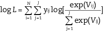 [5.5]
[5.5]
Socio-economic variables can be included along with choice set attributes in the X terms in equation [5.1], but since they are constant across choice occasions for any given individual (e.g. income is the same when the first choice is made as the second), they can only be entered as interaction terms, i.e. interacted with choice specific attributes.
This standard practice of giving respondents a series of choice set cards is not however without its problems. Typically, analysts treat the response to each choice set as a separate data point. In other words, responses for each of the choice sets presented to each respondent are regarded as completely independent observations. This is most probably incorrect, since it is likely that there will be some correlation between the error terms of each group of sets considered by the same individual. The data thus is effectively a panel with n “time periods” corresponding to the n choice sets faced by each individual. Hence, standard models over-estimate the amount of information contained in the dataset. There are procedures to deal with this problem. In some cases an ex post correction can be made by multiplying the standard errors attached to the coefficients for each attribute by the square root of the number of questions administered to each respondent. Other types of model used to estimate DCE data – such the random parameters logit model – automatically correct for this bias within the estimation procedure.
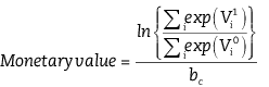
Once the parameter estimates have been obtained, a monetary compensating surplus welfare measure that conforms to demand theory can be derived for each attribute using the formula given by [5.6] (Hanemann, 1984; Parsons and Kealy, 1992) where V0 represents the utility of the initial state and V1 represents the utility of the alternative state. The coefficient bc gives the marginal utility of income and is the coefficient of the cost attribute.
 [5.6]
[5.6]
It is straightforward to show that, for the linear utility index specified in [5.1], the above formulae can be simplified to the ratio of coefficients given in equation [5.7] where bx is the coefficient of any of the (non-monetary) attributes and bc is the coefficient of the cost attribute. These ratios are often known as implicit prices.
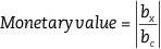 [5.7]
[5.7]
Choice experiments are therefore consistent with utility maximisation and demand theory, at least when a status quo option is included in the choice set.
Notice however that specifying standard errors for the implicit price ratios is more complex. Although the asymptotic distribution of the maximum likelihood estimator for the parameters β is known, the asymptotic distribution of the maximum likelihood estimator of the welfare measure is not, since it is a non-linear function of the parameter vector. One way of obtaining confidence intervals for this measure is by means of the procedure developed by Krinsky and Robb (1986). This technique simulates the asymptotic distribution of the coefficients by taking repeated random draws from the multivariate normal distribution defined by the coefficient estimates and their associated covariance matrix. These are used to generate an empirical distribution for the welfare measure and the associated confidence intervals can then be computed.
Finally, DCE data can be used to estimate the welfare values associated with different combinations of attributes and levels (Bennett and Blamey, 2001). Using the implicit prices estimated for the various attributes allows the researcher to calculate the economic value of particular policy options (defined as specific packages of attributes and levels) in relation to the status quo. Multiple compensating surplus estimates can be derived depending on the levels of the attributes that are selected.
If a violation of the IIA hypothesis is observed, then more complex statistical models are necessary that relax some of the assumptions used. These include the multinomial probit (Hausman and Wise, 1978), the nested logit (McFadden, 1981), the mixed logit or random parameters logit model (Train, 1998), and the latent class model (Boxall and Adamowicz, 2002). IIA can be tested using a procedure suggested by Hausman and McFadden (1984). This basically involves constructing a likelihood ratio test around different versions of the model where choice alternatives are excluded. If IIA holds, then the model estimated on all choices should be the same as that estimated for a sub-set of alternatives (see Foster and Mourato, 2002, for an example).
5.3. Stages of a discrete choice experiment
As described in Section 5.2, the conceptual framework for DCEs assumes that consumers’ or respondents’ utilities for a good can be decomposed into utilities or well-being derived from the composing characteristics of the good as well as a stochastic element. Respondents are presented with a series of alternatives, differing in terms of attributes and levels, and asked to choose their most preferred. A baseline alternative, corresponding to the status quo or “do nothing” situation, is usually included in each choice set. The inclusion of a baseline or do-nothing option is an important element of the DCE approach; respondents are not forced into choosing alternatives they see as worse than what they currently have and so it permits the analysts to interpret results in standard (welfare) economic terms.
A typical DCE exercise is characterised by a number of key stages (Hanley, Mourato and Wright, 2001; Bennett and Blamey, 2001; Bateman et al., 2002; Hoyos, 2010). These are described in Table 5.1.
5.3.1. Example: Measuring preferences for nuclear energy scenarios in Italy
We will illustrate how DCEs work through an example, a recent study of preferences for nuclear energy options in Italy (see Contu, Strazzera and Mourato, 2016, for full details). The planned re-introduction of nuclear energy in Italy was abandoned in the aftermath of the Fukushima nuclear accident, following a referendum that revealed widespread public opposition. But a new “revolutionary” nuclear energy technology, i.e. the fourth generation technology, currently under research and development, is expected to address many of the problems of the current technology, namely minimising the probability of catastrophic accidents as well as the amount of nuclear waste produced. Since nuclear energy remains a key technology in terms of allowing countries to meet their greenhouse gas (GHG) emission reduction targets, it is important to ascertain social acceptance of a new safer nuclear technology.
DCEs were chosen over contingent valuation for the valuation of preferences for nuclear energy. As noted above, DCEs are particularly well suited to value changes that are multidimensional (with scenarios being presented as bundles of attributes) and where trade-offs between the various dimensions are of interest. Nuclear energy scenarios have multiple dimensions that are important to people, some negative and some positive, such as perceived risk of an accident as well as environmental benefits. Second, values are inferred implicitly from the stated choices, avoiding the need for respondents to directly place a monetary value on scenario changes. This latter characteristic has led to suggestions that DCE formats may be less prone to protest responses than contingent valuation as attention is not solely focused on the monetary attribute but on all the scenario attributes (Hanley et al., 2001). This is particularly relevant when dealing with nuclear energy-related scenarios that may be particularly prone to protest votes, given the notoriously strong views held towards nuclear energy by many people.
The choice experiment scenario asked respondents to imagine they had a chance to choose between a series of options regarding the construction of 4th generation nuclear power plants in Italy. The attributes chosen were: GHG emissions reductions (when compared with current emissions, without nuclear technology); nuclear waste reduction (a benefit of the 4th generation nuclear technology when compared with current technology); distance of city of residence from the nuclear power plant (due to safety concerns, living far away from a nuclear power plant is perceived as a benefit); public investments (nuclear power installations are often accompanied by investments in the local area, such as new hospitals and land recovery measures); and electricity bill reductions, per household, per year. The monetary attribute (i.e. bill reductions) is therefore expressed as a monetary compensation. Table 5.2 depicts the attributes and their levels.
Respondents were presented with a series of choice sets and asked to choose their most preferred scenario in each case. Each choice set consisted of a pair of nuclear energy scenarios, containing the five attributes and levels described in Table 2, and a “none” option so that respondents could decide to opt out and choose neither of the two nuclear energy options. Given the five attributes and their levels, with two options per choice task, the total number of possible choice scenarios is 576 (4 distance levels * 4 waste reduction levels * 3 emission reduction levels * 4 bill reduction levels * 3 public investment levels). To reduce the number of choice tasks to present to respondents a main effects orthogonal design was used leading to a total of 64 choice pairs, which were then organised into 8 blocks of 8 choice sets each. For clarity purposes, after piloting, the public investment attribute was presented as two separate attributes: construction of new hospitals (yes or no), and land recovery measures (yes or no). Figure 5.1 depicts an example of a choice set used in the survey.

Discrete choice experiments are consistent with utility maximisation and demand theory, at least when a status quo or opt out option is included in the choice set, as in this case. If a status quo/opt out alternative is not included in the choice set, respondents are effectively being “forced” to choose one of the policy alternatives presented, which they may not desire at all. If, for some respondents, the most preferred option is the current baseline situation (in this case with no nuclear energy), then any model based on a design in which the baseline is not present will yield inaccurate estimates of consumer welfare.
The survey was programmed in Qualtrics and implemented on-line in 2014 on a panel of 1 200 Italian respondents, representative in gender, age and region. Unsurprisingly, the nuclear energy scenarios divided respondents: some 23% of the sample chose none of the nuclear energy scenarios in every single choice set; while a similar proportion always selected one of the nuclear scenarios in every choice instance.
The choice experiment data was analysed employing a conditional logit model, a random parameters model with error components and a latent class model (see Section 5.2). Here we present the results from the conditional logit model. The analysis assumes that the deterministic component of the utility or well-being function Vij (of the ith respondent for the φ different alternatives in the choice set) depends simply (and linearly) on the attributes of the choices presented as follows:
 [5.8]
[5.8]
where βi are the model coefficients, and the remaining variables are the choice experiment attributes as described in Table 5.2. The ASC is an alternative specific constant capturing the variation in choices that is not explained by the attributes. Here it represents the “none” option in each choice set. A positive coefficient b1 will indicate that individuals are more likely to choose none of the nuclear energy scenarios, thereby providing a measure of overall opposition towards nuclear energy. Because of non-linearities, some of the attributes are coded as dummy variables: Distancex (distance of city of residence from the nuclear power plant, dummies for 50, 100 and 200 km, baseline 20 km), Wastex (nuclear waste reduction, dummies for 10, 20 and 30% reduction, baseline “no reduction”) and the public investments Hospitals and Land (construction of hospitals, and land recovery measures respectively, baseline “no investment” in each case). The final two attributes are Emissions (representing atmospheric emission reductions, in 10% intervals) and Bill (representing electricity bill reductions per household, per year, in EUR, obtained by applying the bill reduction percentages to the average of the sampled respondents’ annual electricity bill.
Using the conditional logit model to estimate equation [5.8], the coefficient levels were found to be: b1 = 1.60; b2 = 0.72; b3 = 0.579; b4 = 0.431; b5 = 0.726; b6 = 0.606; b7 = 0.367; b8 = 0.274; b9 = 0.326; b10 = 0.516; b11 = 0.00213. The coefficients on these attributes are all positive as having more of any of these particular things increases utility or well-being, i.e. being located further away from a nuclear power plant, reducing nuclear waste, reducing emissions, investing in new hospitals and land recovery measures, and reducing electricity bills. Moreover, the effect of distance to the nuclear site is non-linear: the magnitude of the coefficients increases with distance.
From these findings the analyst can obtain monetary value estimates by dividing the coefficient of each non-monetary attribute (e.g. b2, the coefficient of Distance 200 km) by the coefficient of the monetary attribute (i.e. b11), as per equations [5.6] and [5.7] above. These values represent willingness to accept compensations, in terms of electricity bill reductions, for a utility-decreasing level of a given attribute (for example, a nuclear power plant situated closer to home); or, alternatively, the willingness to pay (in terms of foregone compensation) for a utility-enhancing level of an attribute (for example, a nuclear power plant situated further away from home, or a reduction in emissions). In this case, as all the attributes are framed in terms of benefits, the valuations can be interpreted as WTP estimates (i.e. foregone compensations). The implicit prices of each attribute are therefore:

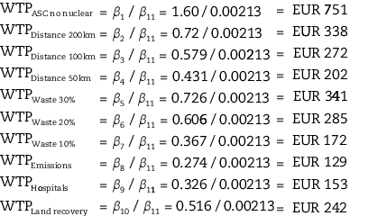
On average, the results show that Italian households are willing to forgo a compensation of EUR 338 per year for a nuclear plant situated 200 km away (vis-à-vis a baseline of 20 km away); this reduces to EUR 202 for a distance of just 50 km. In addition, waste reduction is valued up to EUR 341 (for a 30% reduction), more than land recovery measures (EUR 242) and hospitals (EUR 153). Finally, emission reductions are found to be highly valued at EUR 129 for a 10% reduction. Of note, the ASC representing the status quo, with no nuclear energy, is positive and very highly valued (EUR 751), indicating a broad preference for scenarios not involving nuclear energy.
In 2004, Adamowicz (2004) envisaged a move away from focusing on values for environmental goods to focusing instead on choice behaviour. This prediction seems to have come to fruition: today, DCEs appear to be more popular than CV (Mahieu et al., 2014). Applications abound in transport, health, marketing, agriculture and also environment, both in developed and developing countries. An example of an application in a developing country can be found in Box 5.1.
Tanzanian marine fisheries have suffered a significant decline in biodiversity and productivity in the past three decades. As population and fisher numbers continue to increase, these coastal resources come under increasing pressure. Marine management has generally favoured regulatory solutions such as the establishment of marine protected areas (MPAs), involving total prohibitions on fishing. But MPAs can be inefficient and ineffectual, posing further unrealistic burdens on local low-income fishing communities. PES have the potential to complement existing marine management instruments through the provision of short-term incentives to put up with fishing restrictions – whether they be a spatial or gear restriction – in the form of compensation for loss of catch.
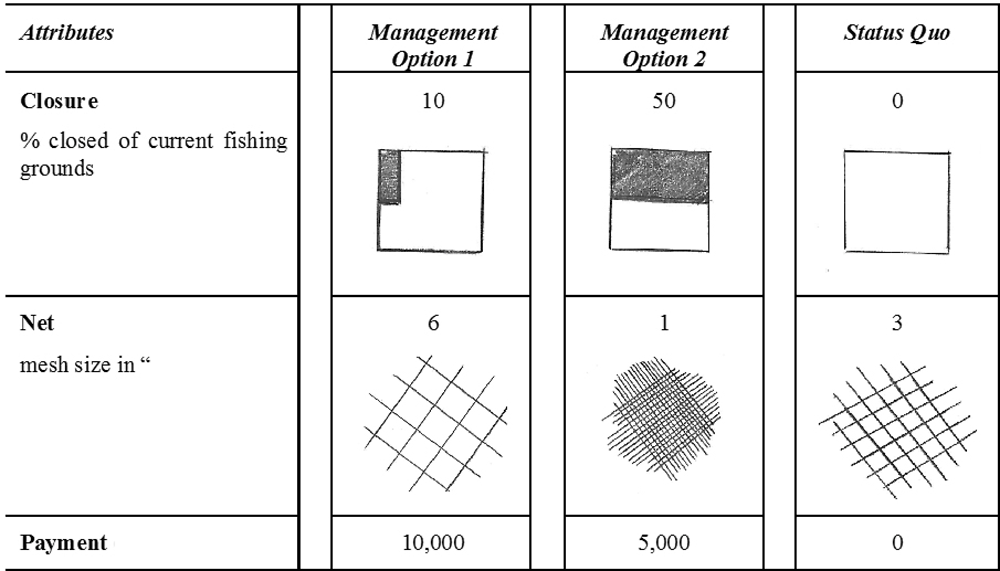
Barr and Mourato (2014) used DCEs to investigate how compensating fishers in Tanzania to adopt restrictions in fishing in a local marine park – through closed areas and gear modifications –, induces participation in a marine PES scheme. Table 3 describes the attributes and levels of the DCE: size of the no-fishing area within the marine park (against a baseline of no spatial restrictions), size of permitted net meshing (where 3mm mesh size was the legal minimum: the wider the meshing the more fish can escape), and monetary compensation. The piloting stages showed a high degree of variation in management attribute preferences. Certain attribute levels (such as a tighter mesh size) were considered highly beneficial to some fishers to the point that they would be willing to pay for it. As such the final monetary attribute included a negative compensation, which is equivalent to a willingness to pay amount.
Given that almost 30% of fishers had no formal education and most of the remaining had only some primary level education, the DCE attributes and levels were depicted visually, using simple black and white drawings (Figure 5.2). Eighteen experimentally designed management scenarios were produced and organised into choice sets. The first two scenario cards were picked at random by the enumerator, without replacement, from a bag containing all 18 scenarios. The status quo baseline scenario was then added, creating a choice set triplet. Each respondent was presented with six of these randomly-generated choice set triplets (Figure 5.2).
Face-to-face interviews were conducted in 2010 with 317 fishers from six coastal villages located in southern Tanzania. The choice data were analysed using a nested logit model. Results show that moving away from the status quo was seen as a significant loss, with fishers requiring an average compensation of USD 12.7 per week (average fishing income in the villages ranged from USD 4.8 to USD 1.3 per day). This was unsurprising given that the status quo was found to be the preferred choice in just over half of the choice sets, with 30% of fishers (96) choosing the status quo in all six choices, revealing aversion to change.
Other results revealed that additional mesh restrictions represented a high utility cost to fishers: weekly compensation amounts of almost USD 10 per fisher were required to move from 3 in. to 6 in. minimum size; while closure of an additional 10% of seascape to fishing activities would require only a compensation of USD 1.60 per week. Fishers appear to equate a 20% closure of fishing grounds as similar in utility loss to that of a 1 in. increase in allowable mesh size. Aggregating the relevant combinations of implicit prices reveals the economic values associated with the various possible PES marine management scenarios, in contrast to the current situation (Table 5.4).
All PES programmes were associated with a high utility loss for fishers, reflecting their aversion to change. The scenario with the lowest restrictions (a closure of just 10% of fishing grounds and maintenance of the current mesh size of 3 in.) reduced fisher utility by USD 14.3 per week (calculated as USD 12.7 to move away from the status quo plus USD 1.60 to put up with the reduction of fishing grounds). As expected, the greatest utility loss was associated with those management options with the greatest restrictions.
Overall, Barr and Mourato (2014) results show an aversion to change and relatively low predicted rates of PES adoption. Approximately only half of the fishers would be willing to sign up for a PES scheme with the lowest restriction of a 10% fishing grounds closure and no change in mesh size. This indicates that the marine PES scheme costs may be high: creating an enabling environment where changes are not met with apprehension and hostility could be as important as investing into conditional in-kind compensation mechanisms.
5.4. Relative strengths and weaknesses of discrete choice experiments
Given that DCEs are a stated preference method, and in effect a generalisation of discrete choice CV, they share many of its advantages and disadvantages. Similar to CV, choice experiments are based on hypothetical scenarios and non-consequential choices with the caveats that this may imply (see Chapter 4). Also like CV, DCEs are very flexible, and are able to measure future changes as well as non-use values. But DCEs have some distinctive characteristics that may differentially affect its performance and accuracy. This section reviews some of the key advantages and disadvantages of DCEs relative to contingent valuation.
5.4.1. Strengths
DCE approaches possess a number of advantages relative to the standard contingent valuation technique (Hanley, Mourato and Wright, 2001; Mahieu et al., 2014). Principal among the attractions of DCEs are claimed to be the following:
-
DCEs are particularly suited to deal with situations where changes are multi-dimensional, and trade-offs between the dimensions are of particular interest, because of their natural ability to separately identify the value of individual attributes of a good or programme, typically supplied in combination with one another. Whilst in principle CV can also be applied to estimate the value of the attributes of a programme, for example by including a series of CV scenarios in a questionnaire or by conducting a series of CV studies, it is a more costly and cumbersome alternative. Hence DCEs do a better job than CV in measuring the marginal value of changes in various characteristics of say environmental programmes, as well as providing a deeper understanding of the trade-offs between them. This is often a more useful focus from a management/policy perspective than focussing on either the overall gain or loss of the good, or on a single discrete change in its attributes. For example, a water company wanting to identify potential areas for investment may need to assess which of the many services they provide are most valued by their customers, and compare those values (i.e. benefits) with the costs of provision. The services provided have multiple dimensions: drinking water quality (e.g. taste and smell of water, hardness of water, water colour, and possible need for boil water notices), reliability of supply (e.g. water pressure, supply interruptions, water leakage, and internal water flooding) and environmental impacts (river water quality, river levels and flow, and possible need for hosepipe bans). Hence, DCEs provide an ideal framework to assess such values.
-
The focus on attributes might increase the potential for generalisation of results making DCEs more appropriate from a value transfer viewpoint (Rolfe, 2006; Rolfe and Windle, 2008). Morrison et al. (1998) provided encouraging early evidence on the use of DCEs in value transfer, highlighting advantages such as allowing for differences in environmental improvements between sites as well as differences in socio-economic characteristics between respondent populations. More recently, Rolf, Windle and Bennett (2015) discuss several reasons why DCEs might lend themselves more easily to value transfer. These reasons relate mostly to the richness and detail of the value estimate output that is produced by DCEs, in terms of multiple attributes and levels. This richness of data is especially relevant when performing benefits transfer using a value transfer function (see Chapter 6 for a discussion of value transfer approaches). The welfare values estimated in DCE studies are a function of both site characteristics and respondent characteristics in the original study site. This same function can then be used for value transfer to a different policy site, using the levels associated with the new site and population’s characteristics, as long as these levels are within the range used in the original study (Rolf, Windle and Bennett, 2015).
-
Insensitivity to the scope of the change is one of the key challengers for CVM (see Chapter 4). In contrast, the simultaneous presentation of the whole and the parts in DCE forces some internal consistency in respondents’ choices. DCEs therefore provide a natural internal (within subjects) scope test due to the elicitation of multiple responses per individual. The internal test is however weaker than an external (between subjects) split-sample scope test in as much as the answers given by any particular individual are not independent from each other and thus sensitivity to scope is to some extent forced. In one of the few existing formal tests of sensitivity to scope in both CV and DCEs, Foster and Mourato (2003) undertook separate CV studies of two nested public goods both of which were explicitly incorporated in a parallel DCE survey. The authors found that, while there was evidence that both CV and DCE produced results which exhibited sensitivity to scope, the evidence for the DCE method was much stronger than that for CV. This result conforms with prior expectations as the scope test used for the CV method was an external test and consequently more demanding than the internal test provided by the DCE method.
-
DCEs are more informative than discrete choice CV studies as respondents get multiple chances to express their preference for a valued good over a range of payment amounts: for example, if respondents are given 8 choice pairs and a “do nothing” option, they may respond to as many as 17 bid prices, including zero. In fact, DCEs can be seen as a generalisation of discrete choice contingent valuation concerning a sequence of discrete choice valuation questions where there are two or more goods involved (Hanley, Mourato and Wright, 2001). When valuing multi-attribute programmes, DCE studies can potentially reduce the expense of valuation studies, because of their natural ability to value programme attributes in one single questionnaire and because they are more informative than discrete choice CV surveys.
-
Choice experiments generally avoid an explicit elicitation of respondents’ willingness to pay (or willingness to accept) by relying instead on choices amongst a series of alternative packages of characteristics from where willingness to pay can be indirectly inferred. As such, DCEs may minimise some of the response difficulties found in CVM such as protest bids, strategic behaviour, or yeah saying (Hanley, Mourato and Wright, 2001). But this point, while intuitive, is speculative and has yet to be demonstrated. In a recent review of DCE studies, Rakotonarivo et al. (2016) find rates of protest ranging from 2% to 58% in developed countries, but since there were no comparative studies performed using CV we cannot say whether CV would have performed any worse.
5.4.2. Weaknesses
Experience with DCEs in environmental contexts and more widely in the fields of transport, marketing and health also highlight a number of potential problems:
-
Arguably, the main disadvantage of DCE approaches lies in the cognitive difficulty associated with multiple complex choices between bundles with many attributes and levels. While the drive for statistical efficiency is improved by asking a large number of difficult trade-off questions, respondents fare better (i.e. response efficiency) when confronted with a smaller number of easier trade-offs (Johnson et al., 2013). Both experimental economists and psychologists have found ample evidence that there is a limit to how much information respondents can meaningfully handle while making a decision. One common finding is that the choice complexity can lead to greater random errors or at least imprecision in responses (see Box 5.2). More generally, since respondents are typically presented with large number of choice sets there is scope for both learning and fatigue effects and an important issue is which – on average – will predominate and when. Handling repeated answers per respondent also poses statistical problems and the correlation between responses in such cases needs to be taken into account and properly modelled (Adamowicz, Louviere and Swait, 1998).
This implies that, whilst the researcher might want to include many attributes and levels, unless very large samples are collected, respondents will be faced with daunting choice tasks. The consequence is that, in presence of complex choices, respondents may use heuristics or rules of thumb to simplify the decision task. These filtering rules lead to options being chosen that are good enough although not necessarily the best, avoiding the need to solve the underlying utility-maximisation problem (i.e. a satisficing approach rather than a maximising one). Heuristics often associated with difficult choice tasks include maximin and maximax strategies and lexicographic orderings (Tversky, 1972; Foster and Mourato, 2002). Hence, it is important to incorporate consistency tests into DCEs studies in order to detect the range of problems discussed above (see, for example, Box 5.2). Section 5 below discusses some recent developments in this area.
-
It is more difficult for DCE approaches to derive values for a sequence of elements implemented by policy or project, when compared with a contingent valuation alternative. Hence, valuing the sequential provision of goods in multi-attribute programmes is probably better undertaken by contingent valuation (Hanley, Mourato and Wright, 2001).
-
In order to estimate the total value of a public programme or a good from a DCEs, as distinct from a change in one of its attributes, it is necessary to assume that the value of the whole is equal to the sum of the parts (see Box 5.1). This raises two potential problems. First, there may be additional attributes of the good not included in the design, which generate utility (in practice, these effects can be captured in other ways). Second, the value of the “whole” may not be simply additive in this way. Elsewhere in economics, objections have been raised about the assumption that the value of the whole is indeed equal to the sum of its parts. This has sometimes been referred to as “package effects” in the grey literature (e.g. eftec and ICS Consulting, 2013). Package effects in DCEs are more likely to be a significant issue when marginal WTP values for changes in attributes are applied to policies involving large and multiple simultaneous changes in attributes, i.e. where substitution effects may be expected.
In order to test whether this is a valid objection in the case of DCEs, values of a full programme or good obtained from DCEs could be compared with values obtained for the same resource using some other method such as contingent valuation, under similar circumstances. In the transport field, research for London Underground and London Buses among others has shown clear evidence that values of whole bundles of improvements are valued less than the sum of the component values, all measured using DCEs (SDG, 1999, 2000). As noted above, Foster and Mourato (2003) found that the estimates from a choice experiment on the total value of charitable services in the UK were significantly larger than results obtained from a parallel contingent valuation survey. They concluded that summing up the individual components of the choice set might seriously overestimate the value of the whole set.
-
A common observation in DCEs is a disproportionate number of respondents choosing the status quo, the baseline, or the opt-out alternative (e.g. Ben Akiva et al., 1991; Meyerhoff and Liebe, 2009). This could reflect status quo bias, i.e. a bias towards the current or baseline situation (Samuelson and Zeckhauser, 1988) that may arise for a number of reasons: inertia, biased perceptions, limited cognitive ability, uncertainty, distrust in institutions, doubts about the effectiveness of the programme proposed, or task complexity (Meyerhoff and Liebe, 2009). A small number of studies authors have experimented with different presentations of the status quo option in DCEs to examine its effects on choice behaviour (Banzhaf, Johnson and Mathews, 2001; Kontoleon and Yabe, 2004).
-
As is the case with all stated preference techniques, welfare estimates obtained with DCEs are sensitive to study design. For example, the choice of attributes, the levels chosen to represent them, and the way in which choices are relayed to respondents (e.g. use of photographs vs. text descriptions, choices vs. ranks) are not neutral and may impact on the values of estimates of consumers’ surplus and marginal utilities.
Contingent ranking is a variant of choice modelling whereby respondents are required to rank a set of alternative options (Hanley, Mourato and Wright, 2001; Bateman et al., 2002), rather than simply choosing their most preferred option as in DCEs. Similarly to DCEs, each alternative is characterised by a number of attributes, offered at different levels, and a status quo option is normally included in the choice set to ensure welfare consistent results. However, the ranking task imposes a significant cognitive burden on the survey population, a burden which escalates with the number of attributes used and the number of alternatives presented to each individual. This raises questions as to whether respondents are genuinely able to provide meaningful answers to such questions. A study by Foster and Mourato (2002) looks at three different aspects of logical consistency within the context of a contingent ranking experiment: dominance, rank consistency, and transitivity of rank order. Each of these concepts are defined below before we proceed to outline the findings of this study:
Dominance: One alternative is said to dominate a second when it is at least as good as the second in terms of every attribute. If Option A dominates Option B, then it would clearly be inconsistent for any respondent to rank Option B more highly than Option A. Dominant pairs are sometimes excluded from choice modelling designs on the grounds that they do not provide any additional information about preferences. However, their deliberate inclusion can be used as a test of the coherence of the responses of those being surveyed.
Rank consistency: Where respondents are given a sequence of ranking sets, it also becomes possible to test for rank-consistency across questions. This can be done by designing the experiment so that common pairs of options appear in successive ranking sets. For example, a respondent might be asked to rank Options A, B, C, D in the first question and Options A, B, E, F in the second question. Rank-consistency requires that a respondent who prefers Option B over Option A in the first question, continues to do so in the second question.
Transitivity: Transitivity of rank order requires that a respondent who has expressed a preference for Option A over B in a first question, and for Option B over C elsewhere, should not thereafter express a preference for Option C over A in any other question. There are clearly parallels here with the transitivity axiom underlying neo-classical consumer theory.
The data set which forms the basis of the tests outlined in Foster and Mourato (2002) is a contingent ranking survey of the social costs of pesticide use in bread production in the United Kingdom. Three product attributes were considered in the survey, each of them offered at three different levels: the price of bread, together with measures of the human health – annual cases of illness as a result of field exposure to pesticides – and the environmental impacts of pesticides – number of farmland bird species in a state of long-term decline as a result of pesticide use. An example choice card for this study is illustrated in Table 5.5.
The basic results of the authors’ tests for logical consistency are presented in Table 5.6. Each respondent was classified in one of three categories: i) “no failure” means that these respondents always passed a particular test; ii) “occasional failures” refers to those respondents who passed on some occasions but not on others; while, iii) “systematic failures” refers to those respondents who failed a test on every occasion that the test was presented.
The results show that on a test-by-test basis, the vast majority of respondents register passes. More than 80% pass dominance and transitivity tests on every occasion, while two thirds pass the rank-consistency test. Of those who fail, the vast majority only fail occasionally. The highest failure rate is for the rank-consistency test, which is failed by 32% of the sample, while only 13% of the sample fails each of the other two tests. Systematic failures are comparatively rare, with none at all in the case of transitivity.
When the results of the tests are pooled, Table 5 indicates that only 5% of the sample makes systematic failures. The overall “no failure” sample accounts for 54% of the total. The fact that this is substantially smaller than the “no failure” sample for each individual test indicates that different respondents are failing different tests rather than a small group of respondents failing all of the tests. Yet, this finding also indicates a relatively high rate of occasional failures among respondents with nearly half of the sample failing at least one of the tests some of the time.
Results such as these could have important implications for the contingent ranking method and choice modelling more generally. The fact that a substantial proportion of respondents evidently find difficulty in providing coherent responses to contingent ranking problems raises some concerns about the methodology, when the ultimate research goal is to estimate coefficient values with which to derive valid and reliable WTP amounts. On the other hand, most errors seem to be occasional, and arguably their frequency should diminish in the simpler setting of a DCE, where only the most preferred alternative (rather than full tanks) need to be identified.
5.5. Recent developments and frontier issues
As stated preference techniques reach maturity, breakthrough developments become less likely. Choice modelling methods have been no exception. Most of the developments in the last decade have been small improvements in statistical design, econometric analysis and in survey implementation methods (with the advent of on-line surveying as discussed in Chapter 4). But there have also been improvements in our understanding of the way individual choices are formulated in sequential choice contexts, as well as developments of new choice model variants. This section provides a brief overview of some of the key developments in understanding respondent behaviour in choice experiment contexts.
5.5.1. Experimental design methods
The selection of the experimental design, i.e. the combination of attributes and levels to be presented to respondents in the choice sets, is a key stage in the development of DCEs, when using fractional factorial designs (Section 2). Recent years have witnessed many developments in experimental design methods (De Bekker-Grob et al., 2012; Johnson et al., 2013). Orthogonal designs (where attributes are statistically independent from one another and the levels appear an equal number of times) are widely used and available from design catalogues, on-line tables of orthogonal arrays, or more commonly from statistical programmes such as SPSS (SPSS, 2008), SPEED (Bradley, 1991), or SAS (Kuhfeld, 2010).
More recently statistically efficient designs (aiming to minimise the standard errors of the parameter estimates for a given sample size) have been developed and are being increasingly used. Amongst these, designs using the D-efficiency criterion are the most common (available in the SAS software). New advanced design software packages designed specifically for DCEs have also been developed in recent years. Specifically, the increasingly popular Ngene (Choice Metrics, 2014) is able to generate designs for a wide range of DCE models, can use Bayesian priors and accommodate specifications with constraints and interaction effects. Finally, as in CV (Chapter 4), web-based surveys have become the most popular way to administer DCEs (Mahieu et al., 2014) and this development has in turn facilitated the implementation of advanced experimental designs.
5.5.2. Understanding response efficiency
The overall precision of parameter estimates in DCE models depends not only on the statistical efficiency of the experimental design discussed in 5.1 but also on response efficiency, i.e. the measurement error that results from respondents’ mistakes and non-optimal choice behaviour (Johnson et al., 2013).
As noted above, it is well known that, in a choice experiment setting, respondents might adopt different processing strategies or heuristics to simplify the choice task (Heiner et al., 1983; Payne et al., 1993). Such aids to the mental thought involved in making a decision in a choice experiment might be a conscious judgement made by the respondent. For example, individuals might rationally choose to make choices considering only a sub-set of the information provided (De Palma et al., 1994). Alternatively, individuals could resort to heuristics (perhaps sub-consciously) due to limited cognitive capabilities or information overload (Simon, 1955; Miller, 1955; Lowenstein and Lerner, 2003).
In line with this, accumulating evidence has been associating different complexity of choice tasks to variations in error variance (Mazzotta and Opaluch, 1995; Dellaert et al., 1999; Swait and Adamowicz, 2001; DeShazo and Fermo, 2002; Arentze et al., 2003; Cassuade et al., 2005; Islam et al., 2007; Bech et al., 2011; Carlsson et al., 2012; Czajkowski et al., 2014; Mayerhoff et al., 2014), suggesting the importance of simultaneously taking into account statistical and respondent efficiency. In other words, respondents could experience fatigue when the choice experiment is complex and/or fail to engage; similarly, the first choice sets might be used by respondents to learn the choice task and employ one, or more, decision rules.
The level of complexity of a choice experiment is defined at the experimental design stage, when the combinations that will be presented to the respondents are determined. On this note, Louviere et al. (2008) provide evidence of a negative relationship between the number of attributes and levels and choice consistency. Concerns regarding respondent efficiency have led to the common practice of dividing the total number of choice sets into smaller blocks so as to reduce the number of choice tasks presented to each respondent (as well as more economical designs to determine the number of these choice sets, such as fractional factorial designs). The blocking procedure can be applied to either a full factorial or to a fractional factorial. The growing attention being given to more flexible and efficient design of DCEs might also help in reducing respondent cognitive burden (see, for example, Severin, 2001; Sándor and Franses, 2009; Danthurebandara et al., 2011).
5.5.3. Non-fully compensatory choice behaviour
It has been widely acknowledged that individuals might present a preference structure which is not as well-behaved as the standard discrete choice models would impose. The standard interpretation of the way in which respondents choose their preferred options in DCEs is that they do so by considering (and trading off) all of the attributes comprising that choice. However, a number of studies have found evidence of departures from this fully compensatory behavior, where respondents may not make such trade-offs and instead make decisions which are non-compensatory, with relatively less preferred attributes never being able to compensate for an attribute that is favoured more. Or perhaps respondents make these trade-offs only partially, making decisions which are semi-compensatory, i.e. it would take a really large amount of some less preferred attribute to compensate for losses in an attribute that respondents favour more. As a result, a wide range of non-compensatory and semi-compensatory decision strategies has been put forward in the literature, to aid the analysis of respondent choices. This has implications in terms of the econometric models employed at the estimation phase as well as at the experimental design phase.
Since the work of Hensher et al. (2005), many studies have been focusing on modelling attribute non-attendance. Attribute non-attendance (ANA) refers to a situation where respondents consider only a subset of the attributes presented in each choice task (i.e. they do not fully trade-off between all the attributes present in the task before them). It has been shown that taking ANA into account might lead to significantly different monetary valuations and/or parameters’ estimates (Hensher, 2006; Hensher and Rose, 2009; Hess and Hensher, 2010; Hole, 2011; Scarpa et al., 2009; Scarpa et al., 2010; Campbell et al., 2011; Puckett and Hensher, 2008; Puckett and Hensher, 2009; Lagarde, 2013).
Attribute non-attendance is usually identified either by directly asking respondents to state whether and which of the attributes they have not considered or, alternatively, inferring this information by means of an appropriate econometric model. Stated ANA was firstly introduced by Hensher et al. (2005); however, it has been questioned as the information obtained poses concerns in terms of its reliability (Campbell and Lorimer, 2009; Carlsson et al., 2010; Hess and Hensher, 2010; Hess et al., 2012; Hess et al., 2013; Kaye-Blake et al., 2009; Kragt, 2013), with some authors putting forward the opposite argument (Hole et al., 2013). As it seems unsatisfactory to crudely discriminate between fully attending and non-fully attending respondents, authors have suggested gathering a more thorough and nuanced information on attribute attendance (Alemu et al., 2013; Colombo et al., 2013; Scarpa et al., 2013). In turn, the inferred ANA literature has proposed that it may be more appropriate to reduce the magnitude of a parameter when there are indications of non-attendance for the corresponding attribute, rather than setting its magnitude equal to zero altogether (Balcombe et al., 2011; Cameron and DeShazo, 2010; Kehlbecher et al., 2013).
Outside of the debate concerning stated ANA versus inferred ANA, other streams of research have been exploring alternative avenues. One example is the concept of stated attribute importance, where respondents are asked to rank the choice experiment attributes in order of importance for their choices (see, for example, Balcombe et al., 2014). Some of this research has also considered the way in which behavioural science might inform how respondent choices are understood. For example, the typical assumption is that a respondent processes choice situations according to a Random Utility Model, where the respondent chooses combinations of attributes within a choice set according to which option provides him or her with the highest utility. However, a respondent’s choice might plausibly reflect other decision procedures such as a Random Regret Model, in which a respondent chooses a preferred option in order to minimise his or her chances of experiencing regret about that choice (Boeri et al., 2012; Chorus et al., 2008, 2014).
Further possibilities exist. Respondents may exhibit lexicographic preferences, where their choice is made according to a strict order based on choosing the option which contains the highest value of a favoured attribute while ignoring other attributes (Sælensminde, 2001; Scott, 2002; Rosenberger et al., 2003; Gelso and Peterson, 2005; Campbell et al., 2006; Lancsar and Louviere, 2006; Hess et al., 2010); while others may use criteria such as Elimination by Aspect (Cantillo and Ortúzar, 2005; Swait, 2001) or reference points (Hess et al., 2012). Finally, the same individual may on some occasions behave according to a full compensatory model, and on other occasions adopt a simplifying strategy (Araña et al., 2008; Leong and Hensher, 2012).
Whether respondents adopt a single or a mixture of decision-making rules depends on the specific case study. What is relevant for the practitioner is that, if heterogeneity in the decision rules used by respondents is present, it should be detected and taken into account when analysing choices in a statistical model. Failure to do so may lead to biased coefficient estimates and, crucially from a policy perspective, monetary valuations. Research is needed so as to identify a set of decision rules which are deemed to best represent the heterogeneity of decision processes whilst still allowing for preference heterogeneity (Hess et al., 2012; Araña et al., 2008; Boeri et al., 2012). Finally, future research still needs to investigate how to interpret or estimate monetary valuations from respondents who exhibit this decisional diversity.
5.5.4. Econometric modelling
Although a sizeable number of studies continues to use the basic conditional logit model (Louviere and Lancsar, 2009), recent reviews of the DCE literature suggest a shift towards more flexible econometric models, that relax some of the restrictive assumptions of the standard model (see Section 2). As noted earlier, researchers have increasingly adopted models such as the nested logit, mixed logit or latent class, that relax the IIA assumption, and importantly better account for preference heterogeneity. In their review of DCE applications in the health field, De Bekker-Grobb et al. (2012) find a small increase in application of these models in the period 2001-2008, when compared with the previous decade. Mahieu et al. (2014) find that the use of more flexible econometric models is more common in environmental research than in health or agricultural research.
The use of advanced econometric models is expected to continue to grow fueled by a number of factors: increased availability of specialist DCE textbooks (e.g. Hensher, Rose and Greene, 2015; Train, 2009); proliferation of DCE courses (e.g. Advanced Choice Modelling Course run by the Centre for Choice Modelling at the University of Leeds; Discrete Choice Analysis course run both at MIT and École Polytechnique Fédérale de Lausanne; Stated Preference Methods: State of the Art Modelling course at the Swedish University of Agricultural Sciences); specialist DCE conferences (e.g. the International Choice Modelling Conference series: www.stata.com).
5.5.5. Best-worst scaling models
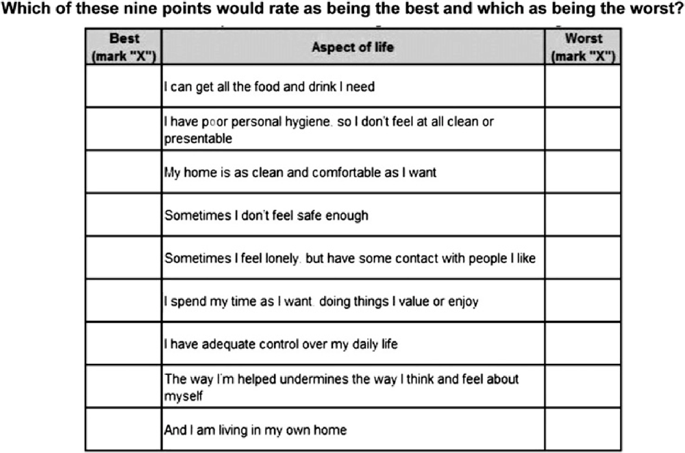
Recently, there has been some interest in the use of Best-Worst Scaling (BWS), an alternative choice-based method that involves less cognitive burden than DCEs. BWS was initially developed by Finn and Louviere (1992), with Marley and Louviere (2005) offering formal proof of its measurement properties. In the BWS approach respondents are presented with a set of three or more items, and asked to choose the two extreme items on an underlying latent scale of interest: best/worst or most/least important, or whatever extremes are appropriate to the study. Respondents are presented with several of these sets, one at a time, and in each case are asked to choose the two extreme items (e.g. the best and the worst) within the set. Experimental design is used to come up with the sets.
Unlike DCEs, in a BWS exercise, respondents are presented with a single scenario at a time, and asked to indicate the best and the worst attribute of that scenario. The aim is to elicit the relative weight or importance that respondents allocate to the various items contained in a set (e.g. attributes of a policy). The focus of the BWS is therefore on preferences for individual attributes rather than scenarios, which sometimes is a useful policy question. However, unless combined with a DCE (e.g. Scarpa et al., 2011), it is not possible to derive monetary values through BWS. BWS is also subject to a number of biases such as position bias (Campbell and Erden, 2015).
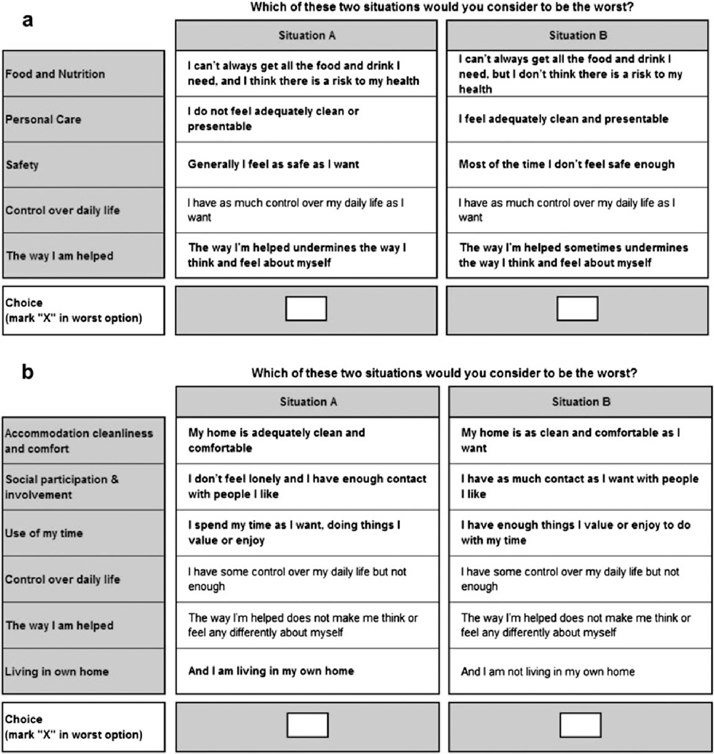
Potoglu et al. (2011) formally compared BWS with a DCE for the same good: social care related quality of life. Figure 5.3 illustrates what the BWS choice set looked like, while Figure 5.4 contains an example of two choice sets used in the parallel DCE. The authors found that both techniques revealed a similar pattern in preferences.
Source: Potoglu et al. (2011).
Source: Potoglu et al. (2011).
The number of applications of BSW has grown in recent years particularly in the field of health (e.g. Flynn et al., 2007). There are also emerging examples in the food, agricultural and environmental literatures (see Campbell and Erdem, 2015, for an overview).
5.6. Conclusions
Many types of environmental impacts are multidimensional in character. What this means is that an environmental asset that is affected by a proposed project or policy often will give rise to changes in component attributes each of which command distinct valuations. This is not unlike the conceptual premise underlying the hedonic approach, a revealed preference method discussed in Chapter 3, where the value of particular goods such as properties can be thought of comprising consumers’ valuations of bundles of characteristics, which can be “teased out” using appropriate statistical analysis. In contrast, however, the suite of stated preference methods known as discrete choice experiments discussed in this chapter must estimate respondents’ valuations of the multiple dimensions of environmental goods, when the good’s total value is not itself observable because no market for it exists. Indeed, it is this information about the (marginal) value of each dimension that is subsequently used to estimate the total value of the change in provision of the environmental good.
While there are a number of different approaches under the choice modelling umbrella, it is arguably the choice experiment variant that has become the dominant approach with regard to applications to environmental goods. In a choice experiment, respondents are asked to choose their most preferred from a choice set of at least two options one of which is the status quo or current situation. This DCE approach can be interpreted in standard welfare economic terms, an obvious strength where consistency with the theory of cost-benefit analysis is a desirable criterion.
Given that DCEs are a stated preference method, they share many of the advantages and disadvantages of the contingent valuation method. Much of the discussion in Chapter 4 about, for example, validity and reliability issues in the context of CVM studies is likely to apply in the context of DCEs. Like CV, choice experiments are based on hypothetical scenarios. Similarly, DCEs are very flexible, and are able to measure future changes as well as non-use values. But, as discussed in this chapter, DCEs also have some distinctive characteristics that may differentially affect its performance and accuracy.
The application of DCE approaches to valuing multidimensional environmental problems has been growing steadily in recent years. DCEs are now routinely discussed alongside the arguably better-known contingent valuation method in state-of-the-art manuals regarding the design, analysis and use of stated preference studies. And in recent years, DCEs appear to have overtaken CV in terms of number of applications and citations (Mahieu et al., 2014) in the fields of environment, agriculture and health. Several factors discussed in this chapter explain the popularity of DCEs. DCE’s are efficient in that they extract extensive information from survey respondents. Their statistical design, implementation and econometric analysis have been facilitated by the development of specialist statistical software and the technology for web surveys, which enables a user-friendly presentation of choice sets to respondents and expedites implementation and analysis considerably. New specialist textbooks, courses, conferences and even a journal (the Journal of Choice Modelling) have helped popularise the method across several disciplines.
Overall, the evidence discussed here seems to point to the superiority of DCEs when valuing complex multidimensional changes. That is, if the focus is on valuing individual components of a policy, and the trade-offs between them are important, then DCEs are possibly the method of choice. Moreover, DCEs are also advantageous when direct elicitation of values might be problematic. But if, instead, we are interested in estimating the total value of a policy then CV would arguably be the preferred method. The choice of method is ultimately case specific, i.e. DCEs should be used when the circumstances demand. As such, whether the two methods should be seen as always competing against one another – in the sense of which is the superior method – is debatable. Both approaches are likely to have their role in cost-benefit appraisals and a useful contribution of any future research would be to aid understanding of when one approach should be used rather than the other. Like CVM, DCEs are very much an important part of the cost benefit analyst’s portfolio of valuation techniques.
References
Adamowicz, W. (2004), “What’s it worth? An examination of historical trends and future directions in environmental valuation”, Australian Journal of Agricultural and Resource Economics, Vol. 48, pp. 419-443, https://doi.org/10.1111/j.1467-8489.2004.00258.x.
Adamowicz, W., J. Louviere and J. Swait (1998), “Introduction to Attribute-Based Stated Choice Methods”, Final Report, NOAA, Washington, DC.
Adamowicz, W. et al. (1998), “Stated Preference Approaches for Measuring Passive Use Values: Choice Experiments and Contingent Valuation”, American Journal of Agricultural Economics, Vol. 80(1), pp. 64-75, https://doi.org/10.2307/3180269.
Alemu, M.H. et al. (2013), “Attending to the reasons for attribute non-attendance in choice experiments”, Environmental and Resource Economics, Vol. 54, pp. 333-359, https://doi.org/10.1007/s10640-012-9597-8.
Araña, J.E., C.J. Leon and M.W. Hanemann (2008), “Emotions and decision rules in discrete choice experiments for valuing health care programmes for the elderly”, Journal of Health Economics, Vol. 27, pp. 753-769, https://doi.org/10.1016/j.jhealeco.2007.10.003.
Arentze, T. et al. (2003), “Transport stated choice responses: Effects of task complexity, presentation format and literacy”, Transportation Research Part E, Vol. 39, pp. 229-244, https://doi.org/10.1016/S1366-5545(02)00047-9.
Balcombe, K. et al. (2014), “Using attribute rankings within discrete choice experiments: An application to valuing bread attributes”, Journal of Agricultural Economics, Vol. 0(2), pp. 446-462, https://doi.org/10.1111/1477-9552.12051.
Balcombe, K.G., M. Burton and D. Rigby (2011), “Skew and attribute non-attendance within Bayesian mixed logit model”, Journal of Environmental Economics and Management, Vol. 62(3), pp. 446-461, https://doi.org/10.1016/j.jeem.2011.04.004.
Banzhaf, M.R., F.R. Johnson and K.E. Mathews (2001), “Opt-Out Alternatives and Anglers’ Stated Preferences”, in Bennett J. and R. Blamey (eds.) (2001), The Choice Modelling Approach to Environmental Valuation, Edward Elgar Publishing Company, Cheltenham, www.e-elgar.com/shop/the-choice-modelling-approach-to-environmental-valuation.
Barr, R. and S. Mourato (2014), “Investigating Fishers’ Preferences for the Design of Marine Payments for Environmental Services Schemes”, Ecological Economics, Vol. 108, pp. 91-103, https://doi.org/10.1016/j.ecolecon.2014.09.006.
Bateman, I.J. et al. (2002), Economic valuation with stated preference techniques: A manual, Edward Elgar, Cheltenham, www.e-elgar.com/shop/economic-valuation-with-stated-preference-techniques?___website= uk_warehouse.
Bateman, I.J. et al. (2009), “Reducing gain-loss asymmetry: A virtual reality choice experiment valuing land use change”, Journal of Environmental Economics and Management, Vol. 58, pp. 106-118, https://doi.org/10.1016/j.jeem.2008.05.003.
Bech, M., T. Kjaer and J. Lauridsen (2011), “Does the number of choice sets matter? Results from a web survey applying a discrete choice experiment”, Health Economics, Vol. 20, pp. 273-286, https://doi.org/10.1002/hec.1587.
Ben-Akiva, M., T. Morikawa and F. Shiroishi (1991), “Analysis of the Reliability of Preference Ranking Data”, Journal of Business Research, Vol. 23, pp. 253-268.
Bennett, J. and R. Blamey (2001), The choice modelling approach to environmental valuation, Edward Elgar, Cheltenham, www.e-elgar.com/shop/the-choice-modelling-approach-to-environmental-valuation.
Bierlaire, M. (2003), “BIOGEME: A free package for the estimation of discrete choice models”, Proceedings of the 3rd Swiss Transportation Research Conference, Ascona, Switzerland.
Boeri, M. et al. (2012), “Site choices in recreational demand: A matter of utility maximization or regret minimization?”, Journal of Environmental Economics and Policy, Vol. 1, pp. 32-47, https://doi.org/10.1080/21606544.2011.640844.
Boxall, P. and W.L. Adamowicz (2002), “Understanding heterogeneous preferences in random utility models: A latent class approach”, Environmental and Resource Economics, Vol. 23, pp. 421-446, https://doi.org/10.1023/A:1021351721619.
Bradley, M. (1991), User’s manual for Speed version 2.1, Hague Consulting Group, Hague.
Cameron, T.A. and J.R. de DeShazo (2010), “Differential attention to attributes in utility-theoretic choice models”, Journal of Choice Modelling, Vol. 3(3), pp. 73-115, www.sciencedirect.com/science/journal/17555345/3.
Campbell, D., C.D. Aravena and W.G. Hutchinson (2011), “Cheap and expensive alternatives in stated choice experiments: Are they equally considered by respondents?”, Applied Economics Letters, Vol. 18, pp. 743-747, https://doi.org/10.1080/13504851.2010.498341.
Campbell, D. and S. Erdem (2015), “Position Bias In Best-Worst Scaling Surveys: A Case Study on Trust in Institutions”, American Journal of Agricultural Economics, Vol. 97(2), pp. 526-545, https://doi.org/10.1093/ajae/aau112.
Campbell, D., W.G. Hutchinson and R. Scarpa (2006), “Lexicographic preferences in discrete choice experiments: Consequences on individual-specific willingness to pay estimates”, Nota di lavoro 128.2006, Fondazione Eni Enrico Mattei, Milano, http://ageconsearch.umn.edu/bitstream/12224/1/wp060128.pdf.
Campbell, D. and V.S. Lorimer (2009), Accommodating attribute processing strategies in stated choice analysis: Do respondents do what they say they do?, 17th Annual Conference of the European Association of Environmental and Resource Economics, Amsterdam, www.webmeets.com/files/papers/EAERE/2009/558/Campbell_Lorimer_EAERE2009.pdf.
Cantillo, V. and J. de D. Ortuzar (2005), “Implication of thresholds in discrete choice modelling”, Transport Reviews, Vol. 26(6), pp. 667-691, https://doi.org/10.1080/01441640500487275.
Carlsson, F. (2010), “Design of stated preference surveys: Is there more to learn from behavioral economics?”, Environmental and Resource Economics, Vol. 46, pp. 167-177, https://doi.org/10.1007/s10640-010-9359-4.
Carlsson, F., M.R. Mørbak and S.B. Olsen (2012), “The first time is the hardest: A test of ordering effects in choice experiments”, Journal of Choice Modelling, Vol. 5(2), pp. 19-37, https://doi.org/10.1016/S1755-5345(13)70051-4.
Cassuade, S. et al. (2005), “Assessing the influence of design dimension on stated choice experiment estimates”, Transportation Research Part B, Vol. 39, pp. 621-640, https://doi.org/10.1016/j.trb.2004.07.006.
ChoiceMetrics (2014), Ngene 1.1.2.: User Manual and Reference Guide. The Cutting Edge in Experimental Design, ChoiceMetrics Pty Ltd.
Chorus, C.G., T.A. Arentze and H.J.P. Timmermans (2008), “A random regret-minimization model of travel choice”, Transportation Research Part B Methodology, Vol. 42, pp. 1-18, https://doi.org/10.1016/j.trb.2007.05.004.
Chorus, C.G., S. van Cranenburgh and T. Dekker (2014), “Random regret minimization for consumer choice modeling: Assessment of empirical evidence”, Journal of Business Research, Vol. 67(11), pp. 2428-2436, https://doi.org/10.1016/j.jbusres.2014.02.010.
Colombo, S., M. Christie and N. Hanley (2013), “What are the consequences of ignoring attributes in choice experiments? Implications for ecosystem service valuation”, Ecological Economics, Vol. 96, pp. 25-35, https://doi.org/10.1016/j.ecolecon.2013.08.016.
Contu, D., E. Strazzera and S. Mourato (2016), “Modeling individual preferences for energy sources: the case of IV generation nuclear energy in Italy”, Ecological Economics, Vol. 127, pp. 37-58, https://doi.org/10.1016/j.ecolecon.2016.03.008.
Czajkowski, M., M. Giergiczny and W. Greene (2014), “Learning and fatigue effects revisited. The impact of accounting for unobservable preference and scale heterogeneity”, Land Economics, Vol. 90(2), pp. 324-351, https://doi.org/10.3368/le.90.2.324.
Danthurebandara, V.M., J. Yu and M. Vanderbroek (2011), “Effect of choice complexity on design efficiency in conjoint choice experiments”, Journal of Statistical Planning and Inference, Vol. 141, pp. 2276-2286, https://doi.org/10.1016/j.jspi.2011.01.008.
De Bekker-Grob, E.W., M. Ryan and K. Gerard (2012), “Discrete choice experiments in health economics: A review of the literature”, Health Economics, Vol. 21, pp. 145-172, https://doi.org/10.1002/hec.1697.
Dellaert, B.G.C., J.D. Brazell and J. Louviere (1999), “The effect of attribute variation on consumer choice consistency”, Marketing Letters, Vol. 10(2), pp. 139-147, https://doi.org/10.1023/A:1008088930464.
De Palma, A., G. Myers and Y. Papeorgiou (1994), “Rational choice under imperfect ability to choose”, American Economic Review, Vol. 84, pp. 419-440.
DeShazo, J.R. and G. Fermo (2002), “Designing choice sets for stated preference methods: The effects of complexity on choice consistency”, Journal of Environmental Economics and Management, Vol. 44, pp. 123-143, https://doi.org/10.1006/jeem.2001.1199.
Eftec and ICS Consulting (2013), South Staffs Water PR14 Stated Preference Study: Final Report, Economics for the Environment Consultancy, London, www.south-staffs-water.co.uk/media/1163/final_report_ ssw_pr14_wtp_study.pdf.
Finn, A. and J.J. Louviere (1992), “Determining the appropriate response to evidence of public concern: The case of food safety”, Journal of Public Policy and Marketing, Vol. 11, pp. 12-25.
Flynn, T.N. et al. (2007), “Best-worst scaling: What it can do for health care research and how to do it”, Journal of Health Economics, Vol. 26, pp. 171-189, https://doi.org/10.1016/j.jhealeco.2006.04.002.
Foster, V. and S. Mourato (2002), “Testing for consistency in contingent ranking experiments”, Journal of Environmental Economics and Management, Vol. 44, pp. 309-328, https://doi.org/10.1006/jeem.2001.1203.
Foster, V. and S. Mourato (2003), “Elicitation format and sensitivity to scope”, Environmental and Resource Economics, Vol. 24, pp. 141-160, https://doi.org/10.1006/jeem.2001.1203.
Gelso, B.R. and J.M. Peterson (2005), “The influence of ethical attitudes on the demand for environmental recreation: Incorporating lexicographic preferences”, Ecological Economics, Vol. 53(1), pp. 35-45, https://doi.org/10.1016/j.ecolecon.2004.01.021.
Green, P. and V. Srinivasan (1978), “Conjoint analysis in consumer research: Issues and outlook”, Journal of Consumer Research, Vol. 5, pp. 103-123.
Greene, W.H. (2008), Econometric Analysis, 6th Edition, Macmillan, New York.
Greene, W.H. (2016), NLogit 6 (software), Econometric Software, Inc.
Hanemann, W.M. (1984), “Discrete/continuous models of consumer demand”, Econometrica, Vol. 52, pp. 541-561.
Hanley, N., S. Mourato and R. Wright (2001), “Choice modelling approaches: A superior alternative for environmental Valuation?”, Journal of Economic Surveys, Vol. 15, pp. 435-462, https://doi.org/10.1111/1467-6419.00145.
Hausman, J. (ed.) (1993), Contingent Valuation: A Critical Assessment, North Holland, Amsterdam.
Hausman, J. (2012), “Contingent valuation: From dubious to hopeless”, Journal of Economic Perspectives, Vol. 26, pp. 43-56, https://doi.org/10.1257/jep.26.4.43.
Hausman, J. and D. Wise (1978), “A conditional Probit model for qualitative choice: discrete decisions recognising interdependence and heterogeneous preferences”, Econometrica, Vol. 42, pp. 403-426.
Hausman, J. and D. McFadden (1984), “Specification tests for the multinomial Logit model”, Econometrica, Vol. 52, pp. 1219-1240.
Heiner, R. (1983), “The origin of predictive behaviour”, American Economic Review, Vol. 73, pp. 560-595.
Hensher, D.A., J.M. Rose and W.H. Greene (2015), Applied Choice Analysis, 2nd edition, Cambridge University Press, New York.
Hensher, D.A., J.M. Rose and W.H. Greene (2005), “The implication on willingness to pay of respondents ignoring specific attributes”, Transportation, Vol. 32, pp. 203-222, https://doi.org/10.1007/s11116-004-7613-8.
Hensher, D.A. (2006), “How do respondent process stated choice experiments? Attribute consideration under varying information load”, Journal of Applied Econometrics, Vol. 21, pp. 861-878, https://doi.org/10.1002/jae.877.
Hensher, D.A. and J.M. Rose (2009), “Simplifying choice through attribute preservation or non-attendance: Implication for willingness to pay”, Transportation Research E, Vol. 45(4), pp. 583-590, https://doi.org/10.1016/j.tre.2008.12.001.
Hensher, D.A. (1994), “Stated preference analysis of travel choices: the state of practice,” Transportation, Vol. 21, pp. 107-133.
Hess, S. and D.A. Hensher (2010), “Using conditioning on observed choices to retrieve individual-specific attribute processing strategies”, Transport Research Part B, Vol. 44, pp. 781-790, https://doi.org/10.1016/j.trb.2009.12.001.
Hess, S., D. Hensher and A.J. Daly (2012), “Not bored yet: Revisiting fatigue in stated choice experiments”, Transportation Research Part A, Vol. 46(3), pp. 626-644, https://doi.org/10.1016/j.tra.2011.11.008.
Hess, S., J.M. Rose and J. Polak (2010), “Non-trading, lexicographic and inconsistent behaviour in stated choice data”, Transportation Research Part D, Vol. 15, pp. 405-417, https://doi.org/10.1016/j.trd.2010.04.008.
Hess, S. et al. (2013), “It’s not that I don’t care, I just don’t care very much: Confounding between attribute non-attendance and taste heterogeneity”, Transportation, Vol. 40(3), pp. 583-607, https://doi.org/10.1007/s11116-012-9438-1.
Hole, A.R. (2011), “A discrete choice model with endogenous attribute attendance”, Economics Letters, Vol. 110, pp. 203-205, https://doi.org/10.1016/j.econlet.2010.11.033.
Hole, A.R., J.R. Kolstad and D. Gyrd-Hansen (2013), “Inferred vs. stated attribute non-attendance in choice experiments: A study of doctors’ prescription behaviour”, Journal of Economic Behavior & Organization, Vol. 96, pp. 21-31, https://doi.org/10.1016/j.jebo.2013.09.009.
Hoyos, D. (2010), “The state of the art of environmental valuation with discrete choice experiments”, Ecological Economics, Vol. 69, pp. 1595-1603, https://doi.org/10.1016/j.ecolecon.2010.04.011.
Islam, T., J.J. Louviere and P.F. Burke (2007), “Modelling the effects of including/excluding attributes in choice experiments on systematic and random components”, International Journal of Research in Marketing, Vol. 24, pp. 289-300, https://doi.org/10.1016/j.ijresmar.2007.04.002.
Johnson, F.R. et al. (2013), “Constructing Experimental Designs for Discrete-Choice Experiments: Report of the ISPOR Conjoint Analysis Experimental Design Good Research Practices Task Force,” Value in Health, Vol. 16, pp. 3-13, https://doi.org/10.1016/j.jval.2012.08.2223.
Kahneman, D. and J. Knetsch (1992), “Valuing public goods: the purchase of moral satisfaction”, Journal of Environmental Economics and Management, Vol. 22, pp. 57-70.
Kanninen, B.J. (ed.) (2007), Valuing Environmental Amenities Using Stated Choice Studies, Springer, Dordrecht.
Kaye-Blake, W.H., W.L. Abell and E. Zellman (2009), “Respondents’ ignoring of attributes information in a choice modelling survey”, Australian Journal of Agricultural and Resource Economics, Vol. 53(4), pp. , https://doi.org/547-564. 10.1111/j.1467-8489.2009.00467.x.
Kehlbacher, A., K. Balcombe and R. Bennet (2013), “Stated attribute non-attendance in successive choice experiments”, Journal of Agricultural Economics, Vol. 64(3), pp. 693-706, https://doi.org/10.1111/1477-9552.12021.
Kontoleon, A. and M. Yabe (2004), “Assessing the Impacts of Alternative ’Opt-out’ Formats in Choice Experiment Studies”, Journal of Agricultural Policy Research, Vol. 5, pp. 1-32.
Kragt, M.E. (2013), “Stated and inferred attribute non-attendance models: A comparison with environmental choice experiments”, Journal of Agricultural Economics, Vol. 64(3), pp. 719-736, https://doi.org/10.1111/1477-9552.12032.
Krinsky, I. and A. Robb (1986), “On approximating the statistical properties of elasticities”, Review of Economics and Statistics, Vol. 68, pp. 715-719.
Kuhfeld, W.F. (2010), Marketing research methods in SAS, SAS Institute Inc Cary. https://support.sas.com/techsup/technote/mr2010.pdf.
Lancaster, K. (1966), “A new approach to consumer theory”, Journal of Political Economy, Vol. 74, pp. 132-157, https://doi.org/10.1086/259131.
Lagarde, M. (2013), “Investigating attribute non-attendance and its consequences in choice experiments with latent class models”, Health Economics, Vol. 22, pp. 554-567.
Lancsar, E. and J. Louviere (2006), “Deleting ’irrational’ responses from discrete choice experiments: A case of investigating or imposing preferences?”, Health Economics, Vol. 15(8), pp. 797-811, https://doi.org/10.1002/hec.2824.
Leong, W. and D.A. Hensher (2012), “Embedding heuristics into choice models: An exploratory analysis”, Journal of Choice Modelling, Vol. 5(3), pp. 131-144, https://doi.org/10.1016/j.jocm.2013.03.001.
Loewenstein, G and J.S. Lerner (2003), “The role of affect in decision making”, in Davidson, R.J., K.R. Scherer and H.H. Goldsmith (eds.) (2003), Handbook of Affective Sciences, Oxford University Press, Oxford.
Louviere, J.J. and D.A. Hensher (1982), “On the design and analysis of simulated choice or allocation experiments in travel choice modelling”, Transportation Research Record, Vol. 890, pp. 11-17.
Louviere, J.J. et al. (2008), “Designing discrete choice experiments: Do optimal designs come at a price?”, Journal of Consumer Research, Vol. 35, pp. 360-375, https://doi.org/10.1086/586913%20.
Louviere, J.J., D.A. Hensher and J.Swait (2000), Stated choice methods: Analysis and applications, Cambridge University Press, Cambridge.
Louviere, J.J. and E. Lancsar (2009), “Choice experiments in health: The good, the bad, and the ugly and toward a brighter future”, Health Economics, Policy, and Law, Vol. 4, pp. 527-546, https://doi.org/10.1017/S1744133109990193.
Louviere, J.J. and G. Woodworth (1983), “Design and analysis of simulated consumer choice or allocation experiments: An approach based on aggregate data”, Journal of Marketing Research, Vol. 20, pp. 350-367.
Luce, R.D. (1959), Individual Choice Behavior: A Theoretical Analysis, John Wiley & Sons, New York.
Mahieu, P.-A. et al. (2014), “Is choice experiment becoming more popular than contingent valuation? A systematic review in agriculture, environment and health”, FAERE Working Paper 2014.12, http://faere.fr/pub/WorkingPapers/Mahieu_Andersson_Beaumais_Crastes_Wolff_FAERE_WP2014.12.pdf.
Marley, A.A.J. and J.J. Louviere (2005), “Some Probabilistic Models of Best, Worst, and Best-Worst Choices”, Journal of Mathematical Psychology, Vol. 49(6), pp. 464-480, https://doi.org/10.1016/j.jmp.2005.05.003.
Mazzotta, M.J. and J.J. Opaluch (1995), “Decision making when choices are complex: A test of Heiner’s hypothesis”, Land Economics, Vol. 71(4), pp. 500-515.
McFadden, D. (1973), “Conditional Logit analysis of qualitative choice behaviour”, in Zarembka, P. (ed.) Frontiers in Econometrics, Academic Press, New York.
McFadden, D. (1981), “Econometric models of probabilistic choice”, in Manski, C. and D. McFadden, (eds.) (1981), Structural Analysis of Discrete Data with Econometric Applications, MIT Press, Cambridge.
Meyerhoff, J. and U. Liebe (2009), “Status Quo Effect in Choice Experiments: Empirical Evidence on Attitudes and Choice Task Complexity”, Land Economics, Vol. 85(3), pp. 515-528.
Meyerhoff, J., M. Oehlmann and P. Weller (2014), “The influence of design dimension on stated choice. An example from environmental valuation using a design of design approach”, Environmental and Resource Economics, Vol. 61(3), pp. 385-407, https://doi.org/10.1007/s10640-014-9797-5%20.
Miller, G.A. (1955), “The magical number seven, plus or minus two. Some limits on our capacity of processing information”, Psychological Review, Vol. 101(2), pp. 343-352.
Morrison, M. et al. (1998), “Choice Modelling and Tests of Benefit Transfer”, Choice Modelling Research Report 8, University College, University of New South Wales, Canberra.
Munro, A. and N. Hanley (1999), “Information, uncertainty and contingent valuation”, in Bateman, I.J. and K.G. Willis (eds.) (1999), Contingent Valuation of Environmental Preferences: Assessing Theory and Practice in the USA, Europe, and Developing Countries, Oxford University Press, Oxford.
Parsons, G.R. and M.J. Kealy (1992), “Randomly drawn opportunity sets in a random utility model of lake recreation”, Land Economics, Vol. 68(1), pp. 93-106.
Payne, J.W., J.R. Bettman and E.L. Johnson (1993), The Adaptive Decision Maker, Cambridge University Press, Cambridge.
Potoglou, D. et al. (2011), “Best-worst scaling vs. discrete choice experiments: An empirical comparison using social care data”, Social Science & Medicine, Vol. 72, pp. 1717-1727, https://doi.org/10.1016/j.socscimed.2011.03.027.
Puckett, S.M. and D.A. Hensher (2008), “The role of attribute processing strategies in estimating the preferences of road freight stakeholders under variable road user charges”, Transportation Research E, Vol. 44(3), pp. 379-395, https://doi.org/10.1016/j.tre.2007.01.002.
Puckett, S.M. and D.A. Hensher (2009), “Revealing the extent of process heterogeneity in choice analysis. An empirical assessment”, Transportation Research Part A: Policy and Practice, Vol. 43(2), pp., https://doi.org/117-126.%2010.1016/j.tra.2008.07.003.
Rakotonarivo, O.S., M. Schaafsma and N. Hockley (2016), “A systematic review of the reliability and validity of discrete choice experiments in valuing non-market environmental goods”, Journal of Environmental Management, Vol. 183, pp. 98-109, https://doi.org/10.1016/j.jenvman.2016.08.032.
Rolfe, J. (2006), “Theoretical issues in using choice modelling data for benefit transfer”, in Rolfe, J. and J. Bennett, (eds.) (2006), Choice Modelling and the Transfer of Environmental Values, Edward Elgar, Cheltenham.
Rolfe, J. and J. Windle, (2008), “Testing for differences in benefit transfer values between state and regional frameworks”, Australian Journal of Agricultural and Resource Economics, Vol. 52, pp. 149-168, https://doi.org/10.1111/j.1467-8489.2008.00405.x.
Rolfe, J., J. Windle and J. Bennett (2015), “Benefit Transfer: Insights from Choice Experiments”, in Johnson, R.J. et al. (eds.) (2015), Benefit Transfer of Environmental and Resource Values: A Guide for Researchers and Practitioners, Springer, Dordrecht.
Rosenberger, R.S. et al. (2003), “Measuring dispositions for lexicographic preferences of environmental goods: Integrating economics, psychology and ethics”, Ecological Economics, Vol. 44, pp. 63-76.
Sælensminde, K. (2001), “Inconsistent choices in stated choice data: Use of the logit scaling approach to handle resulting variance increases”, Transportation, Vol. 28, pp. 269-296.
Samuelson, W. and R. Zeckhauser (1988), “Status Quo Bias in Decision Making”, Journal of Risk and Uncertainty, Vol. 1, pp. 7-59.
Sándor, Z. and H. Franses (2009), “Consumer price evaluations through choice experiments”, Journal of Applied Econometrics, Vol. 24, pp. 517-535, https://doi.org/10.1002/jae.1061.
Scarpa, R. et al. (2011), “Exploring Scale Effects of Best/Worst Rank Ordered Choice Data to Estimate Benefits of Tourism in Alpine Grazing Commons”, American Journal of Agricultural Economics, Vol. 93(3), pp. 813-28, https://doi.org/10.1093/ajae/aaq174.
Scarpa, R., M. Thiene and D.A. Hensher (2010), “Monitoring choice task attribute attendance in non-market valuation of multiple park management services: Does it matter?”, Land Economics, Vol. 86(4), pp. 817-839, https://doi.org/10.3368/le.86.4.817.
Scarpa, R. et al. (2013), “Inferred and stated attribute non-attendance in food choice experiments”, American Journal of Agricultural Economics, Vol. 95(1), pp. 165-180, https://doi.org/10.1093/ajae/aas073.
Scott, A. (2002), “Identifying and analysing dominant preferences in discrete choice experiments: An application in health care”, Journal of Economic Psychology, Vol. 23(3), pp. 383-398.
Steer Davies Gleave (SDG) (1999), Bus Station Passenger Preferences, Report for London Transport Buses, London Transport, London.
Steer Davies Gleave (SDG) (2000), London Underground Customer Priorities Research, Report for London Undergound, London Underground, London.
Severin, V. (2001), Comparing Statistical and Respondent Efficiency in Choice Experiments, Ph.D. Dissertation, Faculty of Economics and Business, the University of Sydney.
Simon, H.A. (1955), “A behavioral model of rational choice”, Quarterly Journal of Economics, Vol. 69, pp. 99-118.
SPSS (2008), Computer software, SPSS Inc Chicago.
Swait, J. and W. Adamowicz (2001), “Choice environment. Market complexity, and consumer behavior: A theoretical and empirical approach for incorporating decision complexity into models of consumer choice”, Organizational behavior and human decision processes, Vol. 86 (2), pp. 141-167, https://doi.org/10.1006/obhd.2000.2941.
Swait, J. (2001), “A non-compensatory choice model incorporating attribute cutoffs”, Transportation Research B, Vol. 35(10), pp. 903-928.
Train, K.E. (1998), “Recreation demand models with taste differences across people”, Land Economics, Vol. 74(2), pp. 230-239.
Train, K.E. (2009), Discrete Choice Methods with Simulation, 2nd Edition, Cambridge University Press, Cambridge.
Tversky, A. (1972), “Elimination by aspects: A theory of choice”, Psychological Review, Vol. 79, pp. 281-299.
Viton, P.A. (2015), Discrete Choice Logit Models with R, Ohio State University, Colombus, http://facweb. knowlton.ohio-state.edu/pviton/courses2/crp5700/5700-mlogit.pdf.