
10. Biodiversity trends in a historical perspective
Biodiversity is important for human well-being as it provides ecosystems services such as the pollination of crops, the prevention of disease, and recreation. This chapter presents historical trends in biodiversity based on multiple indicators. Globally, the average abundance of species population has declined by 44% since 1970. Multiple indicators that cover a long-term timeframe show that biodiversity has declined for the better part of the Holocene, with this trend accelerating since 1900. In the shorter term, efforts to arrest the decline have borne some fruit, with a 36% increase in species abundance in Western Europe since 1970, which contrasts however with an 81% decline in Latin America and the Caribbean. This chapter also puts forward a framework for analysing key drivers of changes in biodiversity. An application of this analytical framework to the case of the Netherlands identifies population growth, intensification of agriculture, expansion of infrastructure and pollution as the key human drivers of biodiversity loss in the country since 1900.
The decline of biodiversity – a term encompassing the variety and variability of life on earth – is one of the most urgent problems facing humanity. Biodiversity is a core feature of an ecosystem that produces human well-being via its positive effects on how ecosystems function. Ecosystems may provide provisioning services such as food and water; regulating services such as floods, drought, land degradation and prevention of disease; supporting services such as soil formation and nutrient cycling; and cultural services such as recreational, spiritual, religious and other non-material benefits. In recent history, economic development, often motivated by aspirations to improve human well-being, has come at the cost of biodiversity loss. Many biologists think that we are currently going through the sixth mass extinction in history, but this time with a very different cause: one species, homo sapiens, is largely responsible for it. Biodiversity loss is the result of complex interactions between humans and nature, and it is happening on an unprecedented scale (Díaz et al., 2019[1]; IUCN, 2008[2]; CBD, 2014[3]; Millennium Ecosystem Assessment, 2005[4]).
Global targets have been set, through the Convention on Biological Diversity (CDB), to significantly reduce the current pace of biodiversity loss (CBD, 2014[3]). Unfortunately, much remains unknown about the extent, rate and causes of the decline in global biodiversity. These knowledge gaps impede our ability to predict and mitigate its impacts. A historical perspective may help to identify events, processes and patterns of biodiversity decline. Processes directly and indirectly associated with declines in biological diversity have largely driven the development of civilisations since the Early- to Mid-Holocene about 5 000-7 000 years ago. These processes include the conversion of natural habitats to agriculture, the unsustainable exploitation of natural resources, the alteration of bio/geochemical cycles, the substitution of native and wild species by exotic and domesticated ones, the appropriation of primary production, and other human activities that generally lead to biodiversity loss (Naeem et al., 2016[5]). Additionally, a historical perspective on biodiversity may help to understand the impact of long-term processes. Short-term events such as cyclical movements of the economy and political changes may have small impacts on biodiversity, while long-term processes such as technological transitions or natural changes may have a more fundamental impact. Thus, better understanding the long-term development of biodiversity may help make better-informed decisions for protecting biodiversity. In a broader context, a long-term perspective may show the benefits of normally functioning ecosystems for human well-being in terms of the services they provide, while also revealing the boundaries of their carrying capacity (van Goethem and van Zanden, 2019[6]).
A multitude of indicators are used today to study (global) biodiversity loss, as biodiversity is a complex concept that is difficult to measure with a single metric (CBD, 2014[3]). Most of these indicators tend to be relatively data-intensive, often relying on extensive field monitoring programmes. This has resulted in two major limitations. First, because of the data availability issues, many indicators only have a species-specific or regional focus; only a few indicators have a country-specific focus. Second, again because of data limitations, these indicators generally go back only to 1970 or cover even shorter time periods. Historical indicators of changes in biodiversity, going back further in time, are scarce. Recently, however, more studies have been using interdisciplinary sources to compile longer and more complete records of developments in biodiversity. Ecologists can provide data on a micro-scale going back some 150 years, while historians can contribute data on a meso-scale up to 2 000 years ago, and archaeologists and paleo-biologists on a macro-scale, covering periods up to 10 000 years ago (Callicott, 2002[7]). Comparing measures from these partially overlapping temporal scales can help characterise historical species occurrence and biodiversity loss. This interdisciplinary approach, although relatively new, has produced some promising results, especially when combined with results from model studies (Kaplan, Krumhardt and Zimmermann, 2009[8]; Seebens et al., 2017[9]).
The set-up and content of this chapter is somewhat different from the other chapters in this book. Historical biodiversity research is a relatively new and heterogeneous field of research. In this chapter, the long-term trends in biodiversity are illustrated based on multiple indicators. Because of data limitations, no country-level data are presented, only data for larger world regions, the world as a whole, or specific ecosystems. Also, many often-used biodiversity indicators have a limited time frame; therefore we present several novel indicators relying on interdisciplinary data. Such indicators generally do not fit the “1820 to now” time frame of this book, as they tend to cover much longer time periods; also they do not refer to individual countries, as do other chapters in this book, but to the world as a whole, or specific ecosystems. Moreover, this chapter presents a case study to explore the relationship between GDP and biodiversity loss in the Netherlands and to identify potential drivers of (changes in) biodiversity. The case study relies on a novel framework that could be applied in future analysis.
The chapter has three sections. The first section presents biodiversity indicators based on the Living Planet Index (LPI) methodology and data for different world regions. These indicators, based on developments of vertebrate populations since 1970, show that globally the abundance of these species populations has declined by 36% between 1970 and 2010, with some regions faring much worse than others. The second section presents a suite of biodiversity indicators sourced from historical research to assess developments in global and regional biodiversity on longer timescales. These indicators, most referring to biodiversity trends well into the Holocene (up to 10 000 years BC), highlight that biodiversity has declined at least since 1500 AD, and probably for the better part of the Holocene. The last section presents a case study reconstructing biodiversity change in the Netherlands from 1900 onwards, showing a long-term decline in biodiversity between 1900 and 1970 and a partial recovery since the 1980s. By analysing specific assemblages of species, this section identifies population growth, the intensification of agriculture, the expansion of infrastructure, and pollution as the key human drivers of biodiversity loss in the Netherlands. The section also highlights an inverted U-curve link between GDP levels and biodiversity loss, which is in line with the environmental Kuznets curve hypothesis. However, the link is not an “automatic” one, suggesting the need for more explicit hypotheses about the mechanisms explaining the link between economic growth and the degradation of nature.
Biodiversity is a complex concept, encompassing the variety and variability of all life on Earth, ranging from the genetic level (i.e. the diversity within a given species) to the species level (i.e. the number of species and the size of their population) and the ecosystem level (i.e. the diversity of ecosystems). This chapter presents evidence on the diversity of species and ecosystems as measured with several indices.
Species diversity usually refers to the number of species present in a certain territory – or in the world as a whole. It is, more or less, known how many vertebrate species have, for example, become extinct globally. Current estimates suggest that, since the year 1500, over 332 terrestrial vertebrates, 150 of them birds, have become extinct (IUCN, 2014[10]). Some authors have suggested that the current extinction rate of all species globally is over 1 000 times faster than the natural “background” rate of around 1-5 per year (Ceballos et al., 2015[11]). Species extinction is, however, only the tip of the biodiversity iceberg. Species abundance (the number of individuals belonging to each species per km2) may be a more meaningful measure of biodiversity, as it can change dramatically over time even when no extinctions occur. Species abundance is therefore often used alongside measures of species richness.
The spatial scope of biodiversity indicators is also important (McGill et al., 2015[12]). Species may become extinct and biodiversity decline at the global level, whereas biodiversity may be stable or even rising at the local level, with certain species – perhaps those best adapted to human influences – becoming more widespread (Dornelas et al., 2014[13]; Dornelas et al., 2019[14]).
Measuring biodiversity is very difficult, especially over large spatial-temporal scales. Assessments therefore tend to look at particular components of biodiversity across terrestrial, marine and other aquatic ecosystems. This may involve species population, extinction risks, habitat extent and condition, and community composition. The suite of biodiversity indicators of the Convention on Biological Diversity (CBD) consider different components of global biodiversity (Table 10.1), divided into indicators of “state”, “pressure” and “response”. Among these categories, only the state indicators cover species diversity directly, albeit at different levels of detail, i.e. species populations, extinction risks and ecosystem level. The pressure indicators assess biodiversity decline only indirectly, by considering some of its key drivers, while the response indicators quantify the (policy) measures used to limit biodiversity decline. However, most indicators in the CBD framework have a relatively short time frame.
The complexity of the concept of biodiversity, and the difficulties that arise when measuring it even today, imply that historical studies can only make use of proxies. Historical sources – in particular when they stretch far back in time – often relate to vertebrates, especially mammals and birds. Historical studies on biodiversity among plants often resort to early taxonomical works.1 One way to overcome the measurement problem is to select “indicator species” that are believed to provide information on the overall status of the ecosystem and on the health of other species in that ecosystem. Such species include umbrella species, whose requirements for persistence include those of an array of associated species; keystone species, on which the health of the ecosystem depends; and foundation species that define much of the structure of a community by creating locally stable conditions for other species. Indicator species may also reflect the quality and changes in environmental conditions and in various aspects of community composition (Lindenmayer, Margules and Botkin, 2000[16]; Siddig et al., 2016[17]). By making a careful selection of indicator species representing the various biological characteristics of ecosystems in a region of a country, one can gain a better understanding of trends of biodiversity, in contexts where data on a broader range of species is lacking. Moreover, the impact of anthropogenic disturbances can be studied by selecting indicator species that are sensitive to environmental change. Indicator species are included in several contemporary indices of biodiversity such as the WWF Living Planet Index, which is based on trends in a limited range of species, most of them birds and mammals (Loh et al., 2005[18]; McRae, Price and Collen, 2012[19]). Applying such an approach in historical research is more complex, as the availability of historical sources is a limiting factor in selecting the appropriate indicator species. Several studies, however, have used indicator species in historical research.
A lively scientific debate has developed revolving around the question of whether economic growth can benefit the environment or instead typically leads to growing environmental problems. The central notion in this discussion is that of the environmental (or green) Kuznets curve, an analogy with Simon Kuznets’s observation that income inequality tended to rise during the early stages of modern economic development and then to decline at later stages, due to a range of offsetting tendencies. This idea of an inverted U-curve linking GDP per capita and income inequality has since the early 1990s been applied in the field of environmental economics, suggesting a similar inverted U-curve between GDP per capita and environmental stress or loss of biodiversity. Some studies found that, during the first stages of industrialisation, pollution levels – for example, for certain emissions (SO2) – had a tendency to increase, whereas beyond a certain income threshold, decline set in – due to government policies, technological changes or changes in the structure of the economy (Grossman and Krueger, 1991[20]). The initial support for this hypothesis has, however, been replaced by a much more critical attitude, as it became clear that for many forms of pollution no “automatic” decline occurs beyond a certain income level (Dinda, 2004[21]; Stern, 2004[22]).
A similar discussion has emerged about the link between economic growth and biodiversity loss. Some authors have argued that a U-shaped relationship between GDP and biodiversity is theoretically impossible, because the extinction of species is an irreversible process and because ecosystems, once destroyed, cannot be reconstructed (Dietz and Adger, 2003[23]; Czech, 2008[24]). Others have found evidence that deforestation is negatively related to GDP levels (evidence that has been criticised by Mills and Waite (2009[25]), or that direct measures of biodiversity – for example, the share of threatened species – show a U-shaped link with GDP (Naidoo and Adamowicz, 2001[26]). McPherson and Nieswiadomy (2005[27]) documented the existence of a U-shaped link for mammals and birds, but not for plants, amphibians, reptiles and invertebrates, for which data are, however, much less satisfactory. Similarly, more recent research has produced mixed results, sometimes confirming a U-shaped relationship (De Santis, 2013[28]) and sometimes finding no evidence for it (see, for example, the comparative study of 50 US states by Tevie, Grimsrud and Berrens (2011[29])).
The limitations of this literature are, however, obvious. No satisfactory data on trends in biodiversity in the medium- and long-term are available to assess the nature of the relationship between biodiversity and GDP per capita. Data used by this research typically relate to, for example, the number of species classified as endangered (which may vary a lot from country to country), or the amount of land under conservation (De Santis, 2013[28]). Moreover, all data relate to recent years – basically the 1990s-2010s period – and lack historical depth for analysing the changing relationships between economic development and biodiversity.
This chapter presents evidence of biodiversity loss based on two main sources and approaches. A case study for the Netherlands is also included to introduce a framework for identifying and analysing key drivers of changes in biodiversity.
Biodiversity indices for world regions
In this section we present biodiversity indices, following the Living Planet Index (LPI) methodology and data, for the different world regions and on a global level. These indices differ in several respects from those included in Grooten and Almond (2018[30]). The main difference is that we derived biodiversity indices for different world regions, while the LPI has not published separate biodiversity trends for world regions, only for biogeographic realms (e.g. the Palearctic). The Living Planet Index (LPI) was developed to measure the state of the world’s biodiversity from 1970 to the present time. It is one of the leading indicators used for assessing global developments in biodiversity. The index uses time-series data to calculate average rates of change in a large number of populations of terrestrial, freshwater and marine vertebrate species (Loh et al., 2005[18]; Collen et al., 2009[31]). The LPI reports how wildlife populations have changed in size – as opposed to the number of animal species that have been lost or gained. The index is not based on a census of all wildlife but rather on a variety of sources such as journals, online databases and government reports. The Living Planet Database (LPD) currently includes time-series data for over 20 000 populations of more than 4 200 mammal, bird, fish, reptile and amphibian species from around the world.
Population data in the Living Planet Database meet several requirements. They refer to single species monitored at a particular location over time. Different types of population abundance data are included in the database, such as full population counts, estimates (e.g. with population size estimated from measured parameters), densities, indices, proxies (e.g. breeding pairs, nests, tracks), measures per unit efforts (e.g. the number of fish caught per net per hour), biomass data (e.g. spawning stock biomass), sample data (e.g. where a proportion of the population is regularly monitored) and occupancy data (e.g. development in species occurrence in grid squares).2 Abundance data feeding the LPI refer to a single species of vertebrate (mammals, birds, fish, reptiles and amphibians) over a period of at least two years, which do not need to be consecutive. When multiple measurements are taken over the course of a year, they were transformed into a single annual value.3
Here, we followed the generalised additive modelling framework to determine the trend in each population time series as described in Loh et al. (2005[18]) and Collen et al. (2009[31]). Average rates of change are then calculated and aggregated to the species level. No weighting system is applied when aggregating indices to the species level and then to the regional level. For the global measure, both weighted and unweighted aggregation methods have been applied. The weighted method gives a higher weight to trends in species-rich world regions (McRae, Price and Collen, 2012[19]). The total number of species per region was calculated from the IUCN Red List of Threatened species database, based on vertebrate species only, as invertebrates, plants and fungi are not sufficiently represented in the dataset. Moreover, on the global scale, disaggregated indices were computed for birds, mammals, reptiles and amphibians to assess whether trends differ among major taxonomic groups (Leung, Greenberg and Green, 2017[32]). Fish species were not included because of limited data availability.
Biodiversity state and pressure indicators based on historical research
This chapter also presents evidence on long-term trends in biodiversity based on historical research. In general, these indicators have used diverse (non-traditional) sources, including archaeological remains and palynological (i.e. plant pollen) data, but also archival records and oral histories, to reconstruct long-term trends in biodiversity: see van Goethem and van Zandem (2019a[33]) for a review of the sources. Most data are available via (disciplinary) global databases, for example the Global Biodiversity Information Facility (GBIF[34]), the Living Planet Index and the Paleobiology Database (PBDB[35]). These databases mainly cover survey data (>70 years), natural history collections and archaeological and paleo-ecological records, and provide information often stretching back centuries or millennia. This information typically refers to proxies of either states or drivers of biodiversity loss, for the world as a whole or for specific types of ecosystems.
Historical sources are in their infancy, and there are no global databases, only national databases, archives and repositories. An exception is the HMAP Data Collection, which contains marine catchment data from historical archives. Historical sources and data are often challenging to gather in major databases, as they may be reported in a variety of languages and dialects, contain disparate information (as they were created for different purposes), or be unavailable in a digital format (or without metadata). In addition to empirical data, several global models have been developed to reconstruct long-term trends in species occurrence and biodiversity. A common feature of all these models is that they are based on assumptions derived from contemporary research, i.e. the assumption that these relations also hold for the past.
Case study: Biodiversity change in the Netherlands, 1900-2010
The main international reference for biodiversity indices is the Living Planet Index (LPI). This is based on a large number of estimates on the historical evolution of population sizes of different species in the (recent) past. The global and national biodiversity indices generally go back only to 1970. In this chapter, we present a case study where a similar approach is applied to the Netherlands going back to 1900. The basis for this national biodiversity index is the population trends of 58 individual mammal, bird and fish species collected from historical censuses, journal articles, reports and other historical sources. Moreover, by identifying – on the basis of the literature about these species – the habitats, threats and feeding types of the species concerned, it is possible to trace the main drivers of changes in the populations of these species. Changes in GDP per capita and the biodiversity index in the Netherlands (1900-2010) can also be analysed against each other.
This index is based on population data of individual mammal, bird and fish species. Population data refer to the abundance of a species for the Netherlands as a whole. Data were collected for each individual species from journal articles and reports. The dataset included not only census data but also proxies of species abundance such as fish landings and hunting records. No modelled population data were included. In total, 58 species were selected to be included in the index: 14 mammals, 14 fish and 30 birds. Of these 58 species, 55 were breeding in the Netherlands in 1900, of which four became extinct (Lesser horseshoe bat, Atlantic sturgeon, Allis shad and Twait shad); two are almost extinct (Atlantic salmon and Spotted ray); and 54 were breeding in the country in 2015, of which three resettled (Eurasian beaver, Grey seal and Wild boar) and two (Great crested grebe and Roe deer) vastly expanded since 1900.
Species representativeness was not an explicit criterion for the selection of species but was treated as a secondary criterion, because of limited data availability. However, these 58 species are spread more or less evenly over the respective species groups in terms of the number of species occurring and species listed in the Red List. Overall, 19% of the mammal species occurring in the Netherlands were selected, 13% for (breeding) birds and 11% for (freshwater) fish. Also, 57% of the selected mammals are Red List species compared to 35% for all mammals in the Netherlands (implying that our estimates for mammals may be biased downward as compared to the entire mammal group). For birds, 40% of our selected species are Red List species compared to 44% for all species. Furthermore, all major habitat types in the Netherlands (17) are represented by at least four typical species, and most habitat types (13) by eight or more species. A general picture of the number of species that have disappeared (locally extinct) and appeared (exotic species) in the 20th century provides a sense of how representative our dataset is. In total, 240 (breeding) bird, 71 mammal and 124 fish species are currently living in the Netherlands. Since 1900, nine bird, three mammal and eight fish species have disappeared from the Netherlands. On the other hand, 35 bird, eight mammal and 16 fish species have settled since 1900 as exotic species.
We collected population data for each individual species for every 5-year interval starting in 1900 until 2015. Some species (12 in total) had data for each year (or most years) in the time period considered. In this case, we computed a moving average of the 5 years around each 5-year interval. However, most species had gaps in the data, either missing data in between different 5-year intervals or missing data for the earliest time period (mostly between 1900 and 1950). In this case, data were inter- and extrapolated.4
For each species, a measure of relative abundance was calculated based on the maximum abundance found for that species. These biodiversity indices were calculated by taking the mean per 5-year interval of the series involved, with the index presented with a 1900 base year. The disaggregated indices (based on taxonomic class, feeding type, etc.) were calculated based on the same procedures as the national biodiversity index, but only including those species relevant for the respective categories. The details and procedures for selecting species, inter- and extrapolation and calculating the indices are explained in more detail in van Goethem and van Zanden (2019[6]).
The data quality of the different indicators over different time periods is assessed in Table 10.3. Data quality is assessed only with respect to the performance of the chosen indicators. Other methodological issues related to the interpretation of the indicators, e.g. representativeness of indicators or the exact definition of biodiversity loss and how to quantify it, are discussed in the results section.
In general, historical data on species occurrence and abundance are often incomplete and sometimes contradictory. In most cases, the best available data are qualitative or semi-quantitative, and often originate from disparate sources. Several biases and limitations in the historical record need to be considered when studying biodiversity data (McClenachan et al., 2015[41]). Observations of species are generally biased toward those with economic or cultural value, while species that are common or have little economic or cultural value are less well recorded. The number of observations available for each species is also rarely consistent across time and space. Finally, certain original documents providing evidence on biodiversity may have been lost, or they may be fragmented or degraded. Early descriptions of the state of biodiversity should not be confused with direct observations, and a lack of written records does not imply historical absence. These biases and limitations hold true for both direct and indirect (i.e. based on proxies) indicators of biodiversity derived from historical records used in this chapter. These limitations hold true for all the indicators presented in the next section.
There are also limitations in modelled indicators. In general, these models are based on (empirical) cause–effect relationships linking environmental drivers with biodiversity impact, for instance increased energy use, land-use change, forestry and climate change (Ten Brink, 2000[42]). Such an approach has two limitations. First, cause-effect relationships are based on contemporary research, assuming that these will also hold for the past, which they might not. Second, the approach is often hampered by the lack of historical data sources on environmental drivers, resulting in models that are often based on a single driver (when multiple drivers are at work). These limitations hold true for the modelled indicators described in the section on “Historical state and pressure indicators”.
Biodiversity indices for world regions
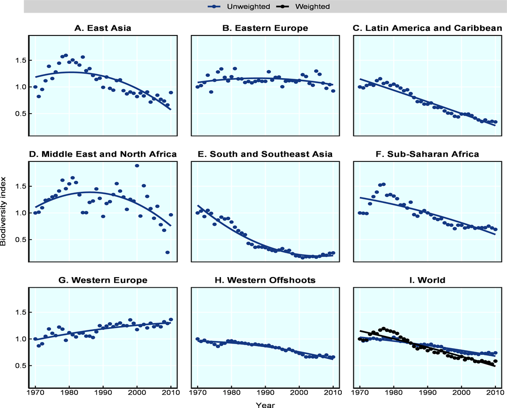
Figure 10.1 and Table 10.4 present biodiversity indices for the different world regions based on the Living Planet Index methodology and dataset. The global index shows that the abundance of a subset of 11 636 populations among 3 701 species has declined by 36% between 1970 and 2010. The indices further indicate that biodiversity loss for these species is much worse in Latin America and the Caribbean and in South and Southeast Asia, with declines of 81% and 75% respectively. Western Europe and Eastern Europe and the former Soviet Union regions, on the other hand, perform much better, with changes limited to 36% and 4%, respectively. Biodiversity loss in other regions is broadly in line with the global index. The disaggregated trends based on taxonomic groups show an average global decline of 21% for mammals, 29% for birds, 48% for reptiles and 44% for amphibians.
The estimates presented in Table 10.3 are average trends. This means that, in the case of the global index, some populations and species are declining by more than 36%, whereas others are not declining as much or are increasing. The average trend calculated for each species in the global biodiversity index shows that just over half of all reptile, bird and mammal species are stable or increasing. Conversely, the trends for over 50% of fish and amphibian species show a decline. As the number of species experiencing a positive or negative trend are, more or less, equal, the average decline for the global index implies that the magnitude of the losses exceeds that of the gains. This also suggests that the fall in the global index is not being driven by losses in just a few very threatened species, but that there are a large number of species in each group (almost 50%) that together produce an average decline.
The 36% decline in biodiversity globally is much less than the 58% decline reported in the Living Planet Index report of 2018 (Grooten and Almond, 2018[30]) (Table 10.4). This difference is explained by the weighting system applied in the 2018 LPI report, which gives a greater weight to species-rich systems, realms and groups. A similar weighting system when applied to our dataset, based on the species richness across world regions, results in a decline of 61%, which is very close to that reported by the LPI. Moreover, the LPI 2012 report provided disaggregated trends based on countries’ income level, ranging from an average increase of 7% for high-income countries to an average decline of 60% for low-income countries (McRae, Price and Collen, 2012[19]). While the LPI country-classification cannot be compared to the one used in this chapter, estimates are very similar in the case of more homogeneous regions, e.g. when comparing Western Europe and high-income countries.5
Biodiversity state and pressure indicators based on historical research
Historical research on global trends in the state of biodiversity suggest that biodiversity has declined at least since 1500, and perhaps for the better part of the Holocene (since 10 000 BC), at least in some world regions (Table 10.2 and Table 10.5). All state indicators show negative trends; three out of the four state indicators on the “pristine” to “late global” timescale show declines since the hunter-gatherer period; and both indicators on the 1500-2000 timescale have been declining since 1500. Additionally, both historical indicators of pressures on biodiversity point to an increase in pressure since the start of each respective period, i.e. since 10000 BC for the ecological footprint, and since 1500 AD for non-native species.
Historical indicators for coral reef ecosystems and for estuaries and coastal seas show similar declines (69% and 76% respectively). According to Pandolfi et al. (2003[36]), coral reef ecosystems experienced a decline in large animals before a decline in small animal species, and Atlantic reefs declined before reefs in the Red Sea and Australia, but the trajectories of decline were markedly similar worldwide. Moreover, all reefs were substantially degraded long before (modern) outbreaks of coral disease and bleaching.
Historical research on the development of estuarine and coastal ecosystems points to similar patterns. (Lotze et al., 2006[37]) report that human impacts have depleted 90% of formerly important species in these ecosystems, destroyed 65% of seagrass and wetland habitat, degraded water quality and accelerated species invasions. All this started long before modern processes of industrialisation and globalisation.
Since 1500, 150 avian extinctions have been identified by historical research on a global scale, with the number of extinctions occurring every 25-year period increasing by 250% from 1500 to 2000. According to Szabo et al. (2012[39]) most losses (78% of species) occurred on oceanic islands, including the Hawaiian Islands, the Mascarene Islands (27 species), New Zealand (22 species) and French Polynesia (19 species), mainly driven by invasive alien species, hunting and agriculture. Ceballos and Ehrlich (2002[38]), reporting on the declining populations as a prelude to species extinction, showed that 173 mammal species across six continents lost over 68% of their historic range area. These declines mostly occurred where human activities are intensive.
The historical indicator on forest coverage in Europe showed an 89% decrease since 1000 BC. Kaplan, Krumhardt and Zimmermann (2009[8]) concluded that humans have transformed Europe’s landscapes since the first agricultural societies in the mid-Holocene. Major impacts were associated with the clearing of forests to establish cropland and pasture, and forest exploitation for fuel wood and construction materials. The human transformation of the landscape also resulted in a decrease of mean species abundance (MSA) of 20% since 1500 and a 5 100% increase of the ecological footprint since 1000 BC. Goldewijk (2014[40])showed that MSA has decreased in all regions of the world, with Europe experiencing a much earlier (and much larger) loss of biodiversity than other regions, mainly due to the loss of almost 90% of its forests. On a global scale, the decline in MSA has been only 20%, because many (larger) countries (e.g. Canada, the United States, Russia, Australia and Brazil) still have a relatively large forest area and high MSA. The historical ecological footprint indicator, on the other hand, increased remarkably in the Holocene, mainly reflecting the expansion of cropland and pasture.
Lastly, Seebens et al. (2017[9]) showed that the first records of non-native species worldwide increased during the last 200 years, with 37% of these increases reported since 1970. The increase can be largely attributed to the diaspora of European settlers in the 19th century, and to the acceleration in trade in the 20th century. For all taxonomic groups, the increase in the number of alien species does not show any sign of saturation, and most groups show increases in the rate of first records over time.
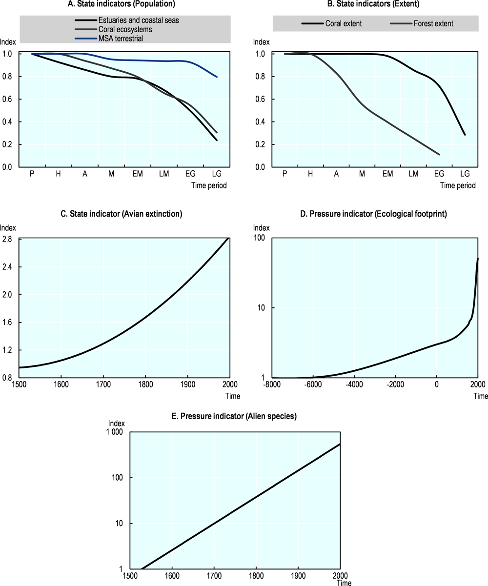
Note: The letters on the horizontal axis of panels A and C stand for: P=Pre-human, H=Hunter-gatherer societies, A=Agricultural societies, M=Medieval times, EM=Early-Modern times, LM=Late-Modern times, EG=Early-Global times, LG=Late-Global times.
Source: Data adapted from papers referenced in Table 10.3.
The development of historical indicators of biodiversity has progressed in recent years. However, there are still considerable gaps and variety in geographic, taxonomic and temporal coverage of the indicators presented in this section. Also, there are gaps for several key aspects of biodiversity states and pressures. Despite this, the available research on key dimensions of biodiversity suggests that, at the global scale, biodiversity has declined for the better part of the Holocene due to human impacts. Compared to Butchart et al. (2010[15]), which present an overview of 31 CBD indicators for the time period between 1970 and 2010, the directions of trends are consistent. The human impact on biodiversity seems, however, to have increased since 1900. Table 10.5 shows that from 30 to 60% of the total change reported by the historical indicators occurred in the last 100 years.
Case study: Biodiversity change in the Netherlands 1900-2010
Figure 10.3 presents a biodiversity index for the Netherlands for 1900-2015. The index shows a long-term decline in biodiversity between 1900 and 1970. The decline starts slowly with industrialisation but gains pace between the 1900s and the 1930s. Around World War II, the decline of biodiversity slows, only to speed up again after the war. The post-war recovery resulted in a strong decline in biodiversity, leading to a low point in the 1970s when biodiversity may have been less than half the level of 1900. Since the 1970s, various protective measures and nature conservation programmes (Cramer, 1989[43]; Leroy, 1994[44]) led to an increase in biodiversity in the mid-1970s that has continued up to the 2010s, while still not recovering to the same level as in 1900. The biodiversity index is based on only vertebrate species; the “state of invertebrate species” is described in Box 10.1.
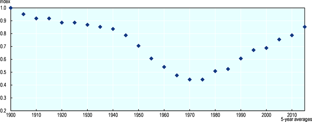
Note: 5-year averages. Based on abundance of 58 species (mammals, birds, fish). Unweighted index.
Source: van Goethem and van Zanden (2019[6]), “Economic development and biodiversity”, CEPR Discussion Paper, No. 13544, https://ssrn.com/abstract=3341351.
Validating our estimates of biodiversity for the Netherlands is complicated, as no other indices describe biodiversity on such a long timescale. It is, however, possible to compare the contemporary part of the index to other indices of biodiversity. Here, the Netherlands national biodiversity index is compared to the Living Planet Index (LPI) for vertebrates in the Netherlands from 1990 to 2015 (van Strien et al., 2016[45]). Our national biodiversity index increases by 39% since 1990 compared to a 22% gain for the LPI. The indices can also be aggregated based on taxonomic class, i.e. birds, mammals, fish. Our biodiversity index shows a 70% increase for mammals as compared to a 123% increase for the LPI for vertebrates; a 29% increase for birds compared to 14% for the LPI; and 33% for fish compared to 14% for the LPI. The recovery in biodiversity in the more recent period is hence consistent with the LPI and with much of the recent research on the development of biodiversity in the Netherlands (van Strien et al., 2016[45]). Also, the data used to derive our biodiversity index are heterogeneous with regards to data type (e.g. including both census data and fish landings) and data quality (some species estimates are partly based on extrapolation). To assess the sensitivity of the results to these issues, subsets of the data were analysed. The sensitivity analysis showed that our biodiversity index (which refers only to vertebrate species) was not much affected by heterogeneity of the data, as the different subsets based on data type and quality yielded similar biodiversity curves both in shape and amplitude. More limited evidence on biodiversity trends for invertebrate species in the Netherlands also points to a continuous decline, see Box 10.1.
The biodiversity trends discussed above relate only to vertebrate species. Hence, they provide a partial picture of the “state of biodiversity”, as only the best-known groups are covered. What about invertebrate species groups? Many invertebrate species have disappeared from the Netherlands; these include species of water insects, bees, butterflies and beetles (Koomen, Van Nieukerken and Krikken, 1995[46]). Recently, several studies have reported on the development of insect populations in Western Europe. Hallmann et al. (2017[47]) found that insects in German nature reserves, particularly macro-moths, ground beetles and Caddisflies, appear to be in severe decline. These datasets suggest a reduction in biomass in macro-moths of approximately 61% and in ground beetles of at least 42%, over a period of 27 years. Van Strien et al. (2019[48]) found that butterflies declined by more than 80% in 1890-2017 on a national level, especially in grassland, woodland and heathland. The trend has stabilised over recent decades in grassland and woodland, but the decline continues in heathland. These studies, albeit limited to only some species groups, suggest that the declines in insects may be a widespread phenomenon.
The observed decline and subsequent increase in biodiversity in the Netherlands can be interpreted by making use of “simple explanations”, such as industrialisation and the emergence of the environmental movement. While these explanations may be largely valid, a more nuanced story can be told by analysing changes in abundance for specific assemblages of species. Figure 10.4 shows aggregate indices based on species type (mammals, fish and birds), habitat preference (urban areas, deciduous forests, open grassland and estuaries) and species threats (pollution, hunting and eutrophication). The indices based on species type (Panel A) show a pattern similar to our national biodiversity index, at least for mammals and birds, and show slightly higher biodiversity in 2015 compared to 1900. Fish species, on the other hand, show a decline, and no recovery in recent years, a pattern that can be explained by the decline of migratory fishes in the second half of the 20th century as a result of damming and water-diversion systems.
Besides species type, the 58 selected species can also be grouped based on types of habitat (Panel B). The index for estuarine species shows a steady decline since 1900, with only a minor recovery since the 1970s low point. The biodiversity levels for these habitats in 2015 are only half those of 1900. Biodiversity in urban areas shows a strong increase since 1900, although this is based on only four species, while biodiversity in open grasslands shows no recovery since 1970. In part, this can be explained by developments in the landscape. Urban areas, for example, saw a six-fold increase compared to 1900. However, the surface area of a certain habitat alone might not explain everything, as habitat quality also needs to be considered, possibly in the case of open grasslands. Biodiversity in forest habitats increased sharply since the second half of the 1970s, partly reflecting a 30% increase in forest surface area.
A more experimental approach is to group species based on the reported causes of decline in the 20th century (Panel C). Qualitative statements on the causes of a decline in abundance have been collected for each species (if applicable) and aggregated into several categories of “species threats”. Species that have endured hunting and persecution show a decline since 1900, with a low point in the 1950s; the level achieved in 2015 is almost 40% higher compared to 1900. In part, this large increase can be explained by the fact that several species (e.g. beaver and grey seal) were extinct in 1900 due to hunting and persecution, but resettled successfully in the 20th century. Moreover, biodiversity levels in 1900 may have been low in general for the species included because of hunting and persecution in the 19th century and even before that time. The eutrophication index shows a steady decrease, with a steady state reached in the 1970s well below the 1900 level. This suggests that eutrophication is still a problem for these species. Here it has to be noted that the index is based on only six species. The pollution index hits a low point around the 1960s and 1970s, with increases ever since, reflecting the banning of many toxic substances since the 1960s.
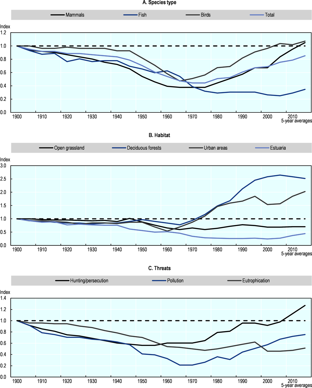
Note: The y-axis runs from 0.2 to 2.6 at 0.2 intervals, the dotted line =1.
Source: van Goethem and van Zanden (2019[6]), “Economic development and biodiversity”, CEPR Discussion Paper, No. 13544, https://ssrn.com/abstract=3341351.
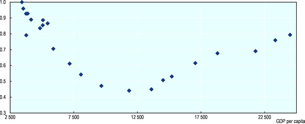
Figure 10.5 plots the development of GDP per capita and the biodiversity index for the Netherlands from 1900 to 2010 (Bolt and van Zanden, 2014[49]). The Pearson correlation coefficients for four time periods are -0.81 (1900-1925), -0.22 (1925-1950), -0.88 (1950-1975) and +0.92 (1975-2010). The negative correlation with GDP per capita from 1900 to 1975 suggests that industrialisation in this period had a strong negative effect on biodiversity. From 1975 onwards, however, the relationship between biodiversity and GDP per capita becomes positive, a pattern that is broadly consistent with the notion of an inverted U-shaped environmental Kuznets curve.
Source: van Goethem and van Zanden (2019[6]), “Economic development and biodiversity”, CEPR Discussion Paper, No. 13544, https://ssrn.com/abstract=3341351.
The working hypothesis underpinning Figure 10.5 is that there is a link between a country’s income level and the protection of nature, but that this link is not an “automatic” one (as assumed in the “naïve” version of the environmental Kuznets curve), but the result of the growth of “green civil society” during economic development, as nature becomes more scarce and the awareness of the need to protect it increases with income growth. The environmental Kuznets curve is therefore a good starting point for this type of research, but the idea has to be supplemented with more explicit hypotheses about the mechanisms that explain the supposed U-turn in the link between GDP and the degradation of nature. There is no reason to assume that economic growth as such leads to such a change.6
A debated issue in biodiversity research is the representativeness of the indices developed, in terms of both indicator type (e.g. richness, diversity) and species selection. In this chapter, the most prominent question is, how representative is the species set on which the biodiversity indices are based. Three main issues can be identified: a skewed distribution of records across regions, across species groups and within-species groups. In general, most datasets are not uniformly distributed across regions and species. For example, birds and mammals are best represented in the LPI dataset, particularly in the Nearctic and Palearctic region, whilst data for other groups are scarce.
One way to deal with the skewed spatial distribution is a weighting approach, which has been developed for the LPI to make the indicator more representative of vertebrate biodiversity. The index is calculated based on a system of weighting that reflects the actual number and distribution of vertebrate species in the world, rather than the number of species present in the dataset. The under-representation of entire species groups, such as insects, is however more difficult to tackle. The IUCN recommended expanding the number of Red List assessments, especially for other species groups, as an important future goal. Besides adding more data, the problem of under-representation can also be tackled by carefully communicating the results, and especially the limitations, of biodiversity research.
The last issue with the representativeness of the data concerns the skewed distribution of records within species groups. The taxonomic catalogues of plants, terrestrial vertebrates, freshwater fish and some marine species are assumed to be sufficient to assess their status and the limitations of our knowledge (Pimm et al., 2014[50]). However, indices based on population trends (particularly at the regional scale) generally include few species that are rare, localised or difficult to survey, including those most susceptible to extinction (Butchart et al., 2004[51]). Also, most species are undescribed. The species we know best have large geographical ranges and are often common within them. Recently, however, Pimm et al. (2014[50]) showed that most newly described species have small ranges and are typically geographically concentrated and disproportionately likely to be threatened or already extinct (Pimm et al., 2014[50]). Therefore, continued attention to representation within species groups is warranted going forwards.
Qualitative and semi-quantitative historical data are essential for deriving longer trends in biodiversity (McClenachan, Ferretti and Baum, 2012[52]). However, a framework for systematically incorporating qualitative information in biodiversity indices is not yet available. This is partly caused by the disparate nature of the data (sources), making it difficult to develop a uniform methodology for matching, or mapping, qualitative information to quantitative data. In our case study for the Netherlands, qualitative data were used conservatively and on a case-by-case basis. In some cases, trends were extrapolated with the help of qualitative information. This approach also has disadvantages, for example, when dealing with historically exploited species that are experiencing recent population increases. (Branch, Matsuoka and Miyashita, 2004[53]) showed, based on data from early 20th century whaling logbooks, that although the population of Antarctic blue whales increased by around 7% per year from 1974 to 2004, it was still below 1% of pre-exploitation abundance levels. This meant that this species should remain protected. Recent population increases are promising, but without data accurately describing the period of exploitation, the magnitude of the recovery can easily be overestimated (Lotze, Coll and Dunne, 2011[54]).
The approach presented in the case study for the Netherlands can be applied to other countries. This would provide an opportunity for a comparative analysis between countries and help to identify relevant drivers of biodiversity across spatial regions and species groups. Also, this would help expand the scope, and analytical depth, of the framework by including quantitative information on drivers of biodiversity, connecting these to the disaggregated biodiversity curves. Moreover, this would provide input to further develop the Kuznets curve hypothesis as a framework, not as the primary driving mechanism, for studying the interaction between biodiversity and socio-economic developments. On a longer timescale, it would be interesting to relate the long-term biodiversity indicators to major socio-economic transitions in human development. Biodiversity research is generally concerned with the present or the recent past. Only short-term processes can be studied in these time frames, while long-term processes are considered, or observed as, boundary conditions (De Vriend, 1991[55]). Long-term biodiversity records may reveal the natural development of biodiversity over ecological timescales, including cycles of succession. The amplitude and frequency of change in these long-term records, or the lack thereof, can be a measure of the impact and scale of disturbances. For example, short-term processes or events can have long-lasting impacts manifested by state shifts of the ecosystem (Scheffer et al., 2001[56]). Perhaps even more interesting is analysing the direction of trends, which might be indicative of socio-economic transitions. These transitions can be characterised by a considerable increase in our species’ impact on the biosphere (Takács-Sánta, 2004[57]). Six such transitions are identified; in chronological order, these are: 1) the use of fire, 2) language, 3) agriculture, 4) civilisation (states), 5) European conquests and 6) the technological-scientific (r)evolution and the dominance of fossil fuels as primary energy sources. Longer time frames may provide an opportunity to study the full impact of human development on biodiversity, as major socio-economic transitions and natural changes come into focus only on these scales.
References
[49] Bolt, J. and J. van Zanden (2014), “The Maddison project: Collaborative research on historical national accounts”, The Economic History Review, Vol. 67/3, pp. 627-651.
[53] Branch, T., K. Matsuoka and T. Miyashita (2004), “Evidence for increases in Antarctic blue whales based on Bayesian modelling”, Marine Mammal Science, Vol. 20, pp. 726-754.
[51] Butchart, S. et al. (2004), “Measuring global trends in the status of biodiversity: Red list indices for birds”, PLoS biology, Vol. 2/12.
[15] Butchart, S. et al. (2010), “Global biodiversity: indicators of recent declines”, Science, Vol. 328/5982, pp. 1164-1168.
[7] Callicott, J. (2002), “Choosing appropriate temporal and spatial scales for ecological restoration”, Journal of Biosciences, Vol. 27/2, pp. 409-420.
[3] CBD (2014), Global Biodiversity, Secretariat of the Convention on Biological Diversity, Montréal, https://www.cbd.int/gbo/gbo4/publication/gbo4-en-hr.pdf.
[38] Ceballos, G. and P. Ehrlich (2002), “Mammal population losses and the extinction crisis”, Science, Vol. 296/5569, pp. 904-907.
[11] Ceballos, G. et al. (2015), “Accelerated modern human-induced species losses: Entering the sixth mass extinction”, Science advances, Vol. 1/5, e1400253.
[31] Collen, B. et al. (2009), “Monitoring change in vertebrate abundance: the Living Planet Index”, Conservation Biology, Vol. 23/2, pp. 317-327.
[43] Cramer, J. (1989), “De groene golf - geschiedenis en toekomst van de Nederlandse milieubeweging”, Utrecht.
[24] Czech, B. (2008), “Prospects for reconciling the conflict between economic growth and biodiversity conservation with technological progress”, Conservation Biology, Vol. 22/6, pp. 1389-1398.
[28] De Santis, R. (2013), “Is there a “Biodiversity Kuznets Curve” for the main OECD countries?”, Rivista di politica economica, Vol. 3, pp. 215-225.
[55] De Vriend, H. (1991), “Mathematical modelling and large-scale coastal behaviour: Part 1: physical processes”, Journal of hydraulic research, Vol. 29/6, pp. 727-740.
[1] Díaz, S. et al. (2019), “Summary for policymakers of the global assessment report on biodiversity and ecosystem services of the Intergovernmental Science-Policy Platform on Biodiversity and Ecosystem Services”, IPBES.
[23] Dietz, S. and W. Adger (2003), “Economic growth, biodiversity loss and conservation effort”, Journal of Environmental Management, Vol. 68/1, pp. 23-35.
[21] Dinda, S. (2004), “Environmental Kuznets curve hypothesis: a survey”, Ecological Economics, Vol. 49/4, pp. 431-455.
[13] Dornelas, M. et al. (2014), “Assemblage time series reveal biodiversity change but not systematic loss”, Science, Vol. 344/6181, pp. 296-299.
[14] Dornelas, M. et al. (2019), “A balance of winners and losers in the Anthropocene”, Ecology Letters, Vol. 22/5, pp. 847-854.
[34] GBIF (n.d.), Free and open access to biodiversity data, Global Biodiversity Information Facility, https://www.gbif.org/.
[44] Glasbergen, P. (ed.) (1994), “De ontwikkeling van het milieubeleid en de milieubeleidstheorie”, VUGA Uitgeverij, Den Haag.
[40] Goldewijk, K. (2014), “Environmental quality since 1820”, in How Was Life?: Global Well-being since 1820, OECD Publishing, Paris, https://dx.doi.org/10.1787/9789264214262-14-en.
[30] Grooten, M. and R. Almond (2018), Living Planet Report - 2018: Aiming Higher, WWF, Gland, Switzerland.
[20] Grossman, G. and A. Krueger (1991), Environmental impacts of a North American free trade agreement, National Bureau of Economic Research.
[47] Hallmann, C. et al. (2017), “More than 75 percent decline over 27 years in total flying insect biomass in protected areas”, PloS one, Vol. 12/10, e0185809.
[10] IUCN (2014), IUCN Red List of Threatened Species. Version 2014.2, http://www.iucnredlist.org.
[2] IUCN (2008), IUCN Red List of Threatened Species. Version 2008, http://www.iucnredlist.org.
[8] Kaplan, J., K. Krumhardt and N. Zimmermann (2009), “The prehistoric and preindustrial deforestation of Europe”, Quaternary Science Reviews, Vol. 28/27-28, pp. 3016-3034.
[46] Koomen, P., E. Van Nieukerken and J. Krikken (1995), Biodiversiteit in Nederland, Nationaal Natuurhistorisch Museum.
[32] Leung, B., D. Greenberg and D. Green (2017), “Trends in mean growth and stability in temperate vertebrate populations”, Diversity and Distributions, Vol. 23/12, pp. 1372-1380.
[16] Lindenmayer, D., C. Margules and D. Botkin (2000), “Indicators of biodiversity for ecologically sustainable forest management”, Conservation Biology, Vol. 14, pp. 941-950.
[18] Loh, J. et al. (2005), “The Living Planet Index: Using species population time series to track trends in biodiversity”, Philosophical Transactions of the Royal Society B: Biological Sciences, Vol. 360/1454, pp. 289-295.
[54] Lotze, H., M. Coll and J. Dunne (2011), “Historical changes in marine resources, food-web structure and ecosystem functioning in the Adriatic Sea, Mediterranean”, Ecosystems, Vol. 14/2, pp. 198-222.
[37] Lotze, H. et al. (2006), “Depletion, degradation, and recovery potential of estuaries and coastal seas”, Science, Vol. 312/5781, pp. 1806-1809.
[41] McClenachan, L. et al. (2015), “The importance of surprising results and best practices in historical ecology”, BioScience, Vol. 65/9, pp. 932-939.
[52] McClenachan, L., F. Ferretti and J. Baum (2012), “From archives to conservation: why historical data are needed to set baselines for marine animals and ecosystems”, Conservation Letters, Vol. 5, pp. 349-359.
[12] McGill, B. et al. (2015), “Fifteen forms of biodiversity trend in the Anthropocene”, Trends in Ecology & Evolution, Vol. 30(2), pp. 104-113.
[27] McPherson, M. and M. Nieswiadomy (2005), “Environmental Kuznets curve: Threatened species and spatial effects”, Ecological Economics, Vol. 55/3, pp. 395-407.
[19] McRae, L., V. Price and B. Collen (2012), The Living Planet Index for Africa.
[4] Millennium Ecosystem Assessment (2005), Ecosystems and Human Well-being: Synthesis, Island Press, Washington, DC.
[25] Mills, J. and T. Waite (2009), “Economic prosperity, biodiversity conservation, and the environmental Kuznets curve”, Ecological Economics, Vol. 68/7, pp. 2087-2095.
[5] Naeem, S. et al. (2016), “Biodiversity and human well-being: An essential link for sustainable development”, Proceedings of the Royal Society B: Biological Sciences, Vol. 283/1844, 20162091.
[26] Naidoo, R. and W. Adamowicz (2001), “Effects of economic prosperity on numbers of threatened species”, Conservation Biology, Vol. 15/4, pp. 1021-1029.
[36] Pandolfi, J. et al. (2003), “Global trajectories of the long-term decline of coral reef ecosystems”, Science, Vol. 301/5635, pp. 955-958.
[35] PBDB (n.d.), ThePaleobiology Database, https://paleobiodb.org/#/.
[50] Pimm, S. et al. (2014), “The biodiversity of species and their rates of extinction, distribution, and protection”, Science, Vol. 344/6187, 1246752.
[56] Scheffer, M. et al. (2001), “Catastrophic shifts in ecosystems”, Nature, Vol. 413/6856, pp. 591-596.
[9] Seebens, H. et al. (2017), “No saturation in the accumulation of alien species worldwide”, Nature Communications, Vol. 8/14435.
[17] Siddig, A. et al. (2016), “How do ecologists select and use indicator species to monitor ecological change? Insights from 14 years of publication in ecological indicators”, Ecological Indicators, Vol. 60, pp. 223-230.
[22] Stern, D. (2004), “The rise and fall of the environmental Kuznets curve”, World Development, Vol. 32/8, pp. 1419-1439.
[39] Szabo, J. et al. (2012), “Global patterns and drivers of avian extinctions at the species and subspecies level”, PloS one, Vol. 7/10, e47080.
[57] Takács-Sánta, A. (2004), “The major transitions in the history of human transformation of the biosphere”, Human Ecology Review, pp. 51-66.
[42] Ten Brink, B. (2000), Biodiversity indicators for the OECD Environmental Outlook and Strategy, RIVM report, Bilthoven, The Netherlands.
[29] Tevie, J., K. Grimsrud and R. Berrens (2011), “Testing the environmental Kuznets curve hypothesis for biodiversity risk in the US: A spatial econometric approach”, Sustainability, Vol. 3/11, pp. 2182-2199.
[33] van Goethem, T. and J. van Zandem (2019a), “Who is afraid of biodiversity? Proposal for a research agenda for environmental history”, Environment and History, Vol. 25/4, pp. 613-647.
[6] van Goethem, T. and J. van Zanden (2019), “Economic development and biodiversity”, CEPR Discussion Paper, No. 13544, https://ssrn.com/abstract=3341351.
[45] van Strien, A. et al. (2016), “Modest recovery of biodiversity in a western European country: The Living Planet Index for the Netherlands”, Biological Conservation, Vol. 200, pp. 44-50.
[48] van Strien, A. et al. (2019), “Over a century of data reveal more than 80% decline in butterflies in the Netherlands”, Biological Conservation, Vol. 234, pp. 116-122.
Notes
← 1. Historical studies on biodiversity among plants often resort to early taxonomical works (and herbals) to get a grip on the species composition in certain areas. Information on species abundances is more difficult to infer from these types of sources. Agricultural statistics and historical maps have been used to estimate these types of indicators.
← 2. Data types that are not used in the database include data from experimental observations (testing different treatments of populations over time), survival rates, recruitment data (such as number of eggs, catches or hunting data, unless they are combined with a measure of effort), or data where survey area or method of data collection has changed over time and has not been corrected for.
← 3. Information on the geographic location and method are included in the LPD. To present an accurate measure of changes in species abundance, both geographical location and method of computation are kept unchanged in each year. If the method of computation changes within the period, the data are entered separately. If only part of the dataset is appropriate for entry, all other values are excluded.
← 4. Data for 10 species relied on interpolation, for 24 species on extrapolation, and for 12 species on a combination of inter- and extrapolation. Linear interpolation was used when data for no more than three consecutive 5-year intervals were missing. When data gaps were larger, additional qualitative information was used. Population data were extrapolated when data were missing for the earliest time period. Extrapolation was based on qualitative and quantitative information from journals, reports and abundance data from later periods. Estimates were made conservatively, e.g. not assuming a linear trend upfront.
← 5. Regional developments by income levels according to the Living Planet Index 2012: Globally, there was a 58% decrease, high-income countries had a 7% increase, middle-income countries had a 31% decrease, and low-income countries had a 60% decrease.
← 6. There is no reason to assume there is an “automatic” environmental Kuznets curve, i.e. that there is a U-turn in the link between GDP and the degradation of nature. Simply put: higher GDP means more production and consumption, which – all other factors remaining equal – implies more pollution, less space for nature and, therefore, biodiversity loss. Changes in the structure of the economy leading to the relative decline of activities that exploit natural resources together with technological change as such (resulting in higher levels of efficiency in using resources) may to some extent help to explain this (Stern, 2004[22]). Moreover, it is important to further explore the “outsourcing” of biodiversity impacts to other countries by moving industrial production abroad. The key to understanding the U-turn, we hypothesise, is changing citizen attitudes towards the environment. The idea is that GDP growth and the increased scarcity of nature will lead to growing concerns about the environment, resulting in the emergence and growth of a “green” civil society. The development of environmental NGOs will in turn lead to increased pressure on the government to introduce and implement environmental policies, for example aimed at the reduction of pollution or the conservation of nature. The quality of the political system is, however, an important intervening variable: will the polity “translate” the bottom-up pressure to carry out green policies into effective measures for the protection of nature?